Recipe
Getting started: embeddings and UMAP
AliPublished
Bio foundation models learn gene and cell context from millions of cells, so their embeddings can capture biological state that PCA on highly variable genes can miss. The Helical MCP lets you run these models from Codex in plain language, then analyse the output in Python.
In this notebook you:
- Install the
helical-platformplugin in Codex and connect it to your Helical account. - Register or select a dataset, then list the available datasets and models.
- Ask Codex to generate and download an embedding.
- Load the embedding into the matching AnnData and plot a UMAP.
1Install the plugin
- The Helical MCP ships in Codex as the
helical-platformplugin, from thehelical-marketplacemarketplace. - To install it from the CLI in a fresh Codex setup, run:
codex plugin marketplace add helicalAI/heli-plugin
codex plugin add helical-platform
- Sign in to Helical when Codex prompts you. The plugin is then ready to use in chat. If you don't have a Helical account yet, create one at console.helical.bio. Your account must be approved before you can use the plugin.
2Register and list datasets and models
- To register a local AnnData file (
.h5ad), ask Codex in plain language:
Register /path/to/your_dataset.h5ad with Helical.
- This example uses
Koenig_10K_ISP, a human heart dataset already in the catalogue, so you only need to list datasets and models.
Dataset list
List the datasets registered in my Helical account.
- Example output (relevant fields):
{
  "rows": [
    {
      "id": "8388af54-090e-4fbc-8008-999c9b1d0484",
      "name": "Koenig_10K_ISP",
      "author": "Koenig",
      "organism": ["Homo sapiens"],
      "tissue": ["heart"],
      "disease": ["DCM"],
      "cellCount": 9925,
      "geneCount": 45068
    }
  ],
  "total": 1
}
Model list
List the available Helical models.
- Helical is model-agnostic: the same workflow runs any of the bio foundation models below, so you can compare them on your data without changing your pipeline.
- Example output, grouped by model family:
| Family | Models |
|---|---|
| Geneformer | gf-6L-10M-i2048, gf-12L-40M-i2048, gf-12L-40M-i2048-CZI-CellxGene, gf-12L-38M-i4096, gf-12L-38M-i4096-CLcancer, gf-12L-104M-i4096, gf-12L-104M-i4096-CLcancer, gf-20L-151M-i4096, gf-18L-316M-i4096 |
| scGPT | scgpt |
| TranscriptFormer | tf_sapiens, tf_exemplar, tf_metazoa |
| Cell2Sentence | c2s_2b |
| Nicheformer | nicheformer |
- The full output also lists the credit cost per cell for each model. To check your balance before a run, ask Codex:
What is my Helical credit balance?
3Generate and download the embedding
- Ask Codex to embed the dataset with your chosen model. This example uses Geneformer
gf-12L-104M-i4096.
Generate embeddings for Koenig_10K_ISP using gf-12L-104M-i4096.
- Review and approve the run when prompted.
- When it finishes, ask Codex to download the embedding to a folder of your choice.
Download the embeddings you generated with the Helical MCP to /path/to/embeddings/koenig.
- Example output from a completed run:
Run: mcp-2026-09-14T13-23-26-822Z-ys3anb (succeeded)
Model: gf-12L-104M-i4096
Artifact: gf-12L-104M-i4096.npy (30,489,728 bytes)
Saved to: /path/to/embeddings/koenig/gf-12L-104M-i4096.npy
- Important: load the original AnnData in its original cell order, attach the embedding, then subset if needed.
4Make the UMAP in Python
- Load the same original AnnData file (
.h5ad) that was embedded. - Keep its cell order unchanged until the embedding is attached.
In [1]:
import scanpy as sc
import numpy as np
4a. Load the source AnnData
- Use the same original
.h5adfile that was embedded.
In [2]:
# Replace with the path to the .h5ad file you embedded
adata = sc.read("/path/to/Koenig_10K_ISP.h5ad")
4b. Check the annotations (optional)
- Run this cell to inspect the object and find valid
obscolumns for plotting.
In [3]:
print(adata)
print("\nAvailable obs columns:")
print(list(adata.obs.columns))
4c. Attach the embedding
- The shape check confirms that there is one embedding vector per cell.
- The embedding is stored in
adata.obsmunder a model-specific key.
In [4]:
# Replace with the path you downloaded the embedding to
embedding = np.load("/path/to/embeddings/koenig/gf-12L-104M-i4096.npy")
assert embedding.shape[0] == adata.n_obs, (embedding.shape, adata.shape)
adata.obsm['X_gf-12L-104M-i4096'] = embedding
print(f"Attached embedding: {embedding.shape}")5Build the neighbour graph and UMAP
- Build neighbours from the Helical embedding.
- Calculate UMAP using that neighbour graph.
In [5]:
sc.pp.neighbors(
    adata,
    use_rep="X_gf-12L-104M-i4096",
    n_neighbors=15,
    metric="cosine",
    key_added="gf-12L-104M-i4096_neighbors",
    random_state=42
)

sc.tl.umap(adata, random_state=42, neighbors_key="gf-12L-104M-i4096_neighbors")6Plot the UMAP
- Colour the UMAP using columns in
adata.obs.
-
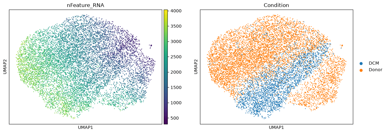
nFeature_RNA: a technical QC covariate (genes detected per cell). If clusters line up neatly with this, your structure may be driven by sequencing depth rather than biology. -
Condition: a biological covariate. This is the signal you actually care about. -
Try another column printed in
adata.obs.columns, or pass a gene name to colour by expression.
In [6]:
sc.pl.umap(adata, color=["nFeature_RNA", "Condition"])
7Save your result
- Keep the embedding and UMAP by saving the AnnData object:
adata.write("koenig_with_helical_embedding.h5ad")