Recipe
Benchmarking bio foundation model embeddings with scIB
When you merge single-cell data from different donors, sites or studies, two goals pull against each other. You want to remove technical variation (which donor it was, which site ran the assay) and keep biological variation (which cell type this is). If you only score the first, a random projection wins. If you only score the second, doing nothing wins.
Bio foundation models like scGPT and Geneformer are trained on tens of millions of cells. The idea is that they have already learned enough about what a cell type looks like to give you embeddings that hold up across batches. Running them yourself means getting the model weights, a GPU, and a preprocessing pipeline that matches what each model expects. The Helical MCP handles that part.
In this cookbook, you compute zero-shot embeddings from scGPT and Geneformer-104M through the Helical MCP, then score them with scIB, a standard benchmark for data integration. The task is scIB's pancreas dataset: 16,382 human pancreas cells sequenced with nine different protocols. You use the 10,963 cells from the five protocols that store raw counts.
- Download the scIB pancreas dataset and prepare it for Helical.
- Register it and get a quote for both models.
- Run the embeddings and download them.
- Score them with scIB against an unintegrated baseline.
- Plot UMAPs.
You need the Helical MCP connected (see Getting started) and about 1 credit.
1Download and prepare the dataset
- The scIB tasks are published as preprocessed AnnData files on figshare.
- The pancreas file needs two fixes before a foundation model can use it:
Xis log-normalised. Both models expect raw counts, and those are stored inlayers["counts"].- Four protocols don't store raw counts. celseq, celseq2, fluidigmc1 and smarter hold non-integer values in
layers["counts"]. For simplicity, drop them and keep the five protocols that store whole numbers (smartseq2 and inDrop1 to inDrop4).
Example prompt:
Download the pancreas dataset from the scIB benchmark figshare and get it ready for Helical. X is log-normalised, so use the counts layer. Keep only the protocols whose counts are all whole numbers. Tell me if anything else looks off.
- Output: a Helical-ready
.h5adwith raw counts: 10,963 cells, 19,093 genes, 5 protocols (tech) and 14 cell types (celltype). - Important: check that the gene names are all symbols. Geneformer requires every entry in the gene index to be a gene symbol, so an index that mixes symbols with Ensembl IDs makes the Geneformer run fail. scGPT runs on the same file.
2Register the dataset and get a quote
Example prompt:
Register the prepared pancreas dataset to the Helical Platform and quote me what it costs to embed with scGPT and Geneformer-104M.
- When the upload finishes, the platform reads the file back and returns the cell and gene counts. Check they match step 1: that confirms the upload arrived intact.
- The quote uses each model's
credits_per_cellrate:
| Model | Credits per cell | Total |
|---|---|---|
| scGPT | 0.000018 | 0.20 |
| Geneformer-104M | 0.000033 | 0.36 |
- Nothing has run yet, and nothing has been charged.
3Run the embeddings
Example prompt:
Run both embeddings, tell me when they're done, and download them to ./embeddings/pancreas.
- Review and approve each run when prompted. Runs only start after you approve them.
- scGPT took about 4 minutes and Geneformer-104M about 7.
- You get one
.npymatrix per model. The rows are in the same order as the cells in the registered dataset, so they line up with thetechandcelltypelabels in your local file.
4Score with scIB
- Score the embeddings with
scib-metrics. - Include a baseline with no batch correction: the first 50 principal components of the log-normalised
X, computed on 2,000 highly variable genes selected per protocol. It gives each score a reference point.
Example prompt:
Score both embeddings with scIB metrics. As a baseline, add a 50-component PCA of the log-normalised X on 2,000 highly variable genes selected per protocol. Batch is tech and label is celltype. One table.
- Output (higher is better for every metric):
| Embedding | Isolated labels | KMeans NMI | KMeans ARI | Silhouette label | cLISI | BRAS | iLISI | kBET | Graph connectivity | PCR | Batch correction | Bio conservation | Total |
|---|---|---|---|---|---|---|---|---|---|---|---|---|---|
| Unintegrated PCA (baseline) | 0.643 | 0.775 | 0.543 | 0.586 | 1.000 | 0.660 | 0.010 | 0.222 | 0.880 | 0.000 | 0.355 | 0.710 | 0.568 |
| scGPT | 0.562 | 0.557 | 0.335 | 0.570 | 0.997 | 0.652 | 0.090 | 0.286 | 0.801 | 0.000 | 0.366 | 0.604 | 0.509 |
| Geneformer-104M | 0.712 | 0.576 | 0.409 | 0.524 | 1.000 | 0.362 | 0.029 | 0.126 | 0.764 | 0.000 | 0.256 | 0.644 | 0.489 |
- Read batch correction and bio conservation separately. Total combines them 40/60 and hides which one you're getting.
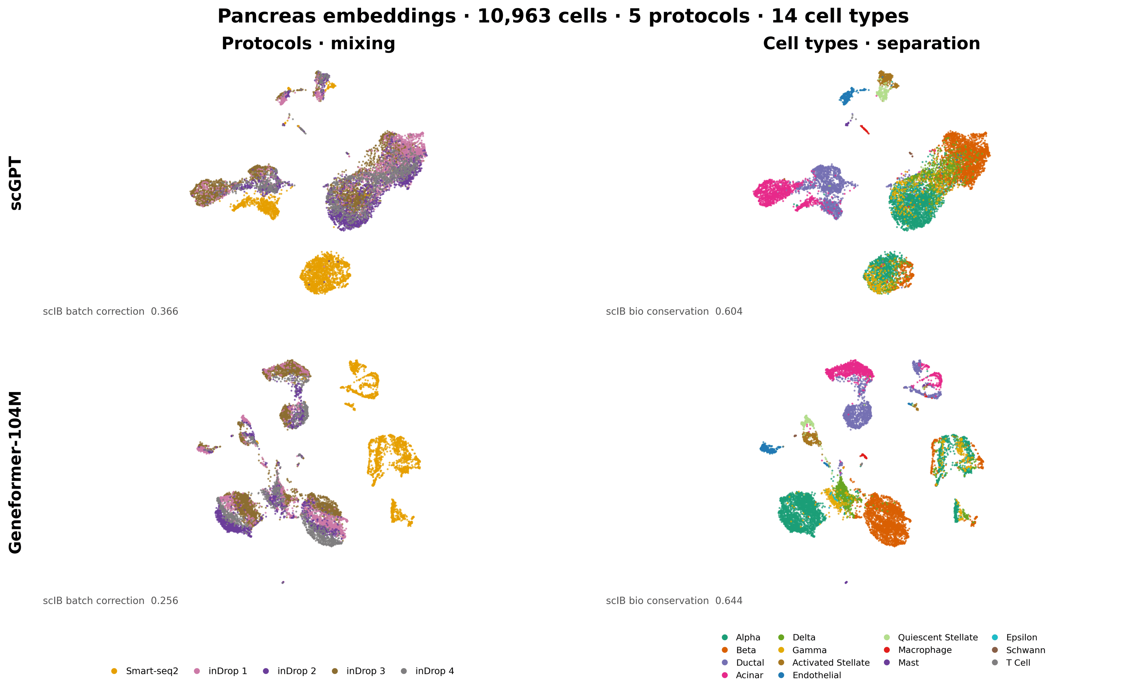
- On this dataset, scGPT scores highest on batch correction and Geneformer-104M on isolated labels. The baseline scores highest on bio conservation.
- iLISI is low for all three, so the protocols stay largely separate in every embedding.
- Notes on the scores:
- PCR is 0 for all three. The baseline is the unintegrated reference that PCR compares against, and scib-metrics caps PCR at 0 when an embedding explains more batch variance than that reference.
- The 7-cell t_cell group is left out of kBET because it is too small.
5Plot UMAPs
Example prompt:
Make UMAPs for each model, coloured by tech and by celltype, so I can see whether the protocols mixed and whether the cell types stayed distinct. Save them as PNG, PDF and SVG.
- Output: figures like the one at the top of this page.
- In both models, the four inDrop runs mix with each other, while Smart-seq2 cells form their own groups. The figure shows the same result as the table.
Takeaways
- The Helical MCP handles the model-specific work (loading weights, preprocessing, running on a GPU). You still decide which data goes in and how to score what comes out.
- The workflow is the same for every model on the platform. To add another model to the comparison, change the model name in the prompts for steps 2 and 3 and rerun the scoring.
- Score a baseline next to the models, so each number has a reference point.
- Check the data before you embed it: which layer holds raw counts, whether those counts are whole numbers in every batch, and whether the gene names are all symbols.
- This benchmark is one of many computational experiments you can run in Helical, the virtual AI lab for biology.
References
- Luecken MD, et al. Benchmarking atlas-level data integration in single-cell genomics. Nature Methods 2022;19:41–50. 10.1038/s41592-021-01336-8
- Preprocessed scIB task data: 10.6084/m9.figshare.12420968