Recipe
Benchmarking scFM embeddings on a clinical label
Immune checkpoint inhibitors (ICIs) treat cancer by boosting the immune system, but in some patients the immune system also attacks the liver. Ji et al. collected blood from patients after ICI treatment, and some of them developed liver injury. Because the injury is immune-driven, the blood may carry the signal: can we predict it from bulk RNA-seq?
Single-cell foundation models usually look at single-cell resolution samples and are evaluated on how well they recover cell identity. Here we apply them to bulk RNA-seq of blood (PBMC), one profile per patient, and ask a slightly different question: can foundation-model use samples from patient's blood to predict a clinical outcome better than traditional methods such as PCA?
In this cookbook we use the Helical MCP to embed a cohort with all 15 foundation models in the catalogue, add a locally computed PCA baseline, and rank every representation by how well logistic regression predicts the clinical label under leave-one-batch-out cross-validation. We then read the paper's own biomarkers off the winning embedding. The data are post-treatment PBMC samples from the checkpoint inhibitor-induced liver injury (ChILI) study of Ji et al.: 59 samples (22 ChILI, 37 ICI-treated controls), 10,000 highly variable genes, 5 sequencing batches.
- Find the dataset and the model catalogue.
- Run all 15 embeddings and add a PCA baseline.
- Explore all 16 representations in one interactive UMAP grid.
- Predict the clinical group, cross-validated by batch.
- Read genes and published biomarkers off the winning embedding.
It takes 6 prompts and around 15 minutes. The steps below go through it one prompt at a time.
You need the Helical MCP connected (see Getting started) and 0.0277 credits, which is what embedding 59 samples with all 15 models costs.
1Find the dataset and the models
listDatasets returns the datasets the account can run against and listModels the foundation-model catalogue with each model's credits_per_cell, so a run can be costed before it is triggered: cells × passes × rate, one pass for an embedding. Neither call spends credit.
Example prompt:
Connect to the Helical MCP. List the single-cell datasets available and the scFM models available.
| Family | Models | Credits per cell | Cost for 59 samples |
|---|---|---|---|
| scGPT | scgpt | 0.000018 | 0.00106 |
| Geneformer | gf-6L-10M-i2048, gf-12L-40M-i2048, gf-12L-40M-i2048-CZI-CellxGene, gf-12L-38M-i4096, gf-12L-38M-i4096-CLcancer, gf-20L-151M-i4096, gf-12L-104M-i4096, gf-12L-104M-i4096-CLcancer, gf-18L-316M-i4096 | 0.000018 to 0.000054 | 0.01457 |
| TranscriptFormer | tf_metazoa, tf_sapiens, tf_exemplar | 0.000037 to 0.000043 | 0.00720 |
| Cell2Sentence | c2s_2b | 0.000063 | 0.00372 |
| Nicheformer | nicheformer | 0.000020 | 0.00118 |
| All 15 models | 0.02773 |
At 0.0277 credits for the whole catalogue, pre-selecting models costs more judgement than compute, so we take all 15. Re-read listModels before quoting your own run: the catalogue is live, and both its membership and its rates change.
2Run the embeddings, then add a PCA baseline
Download the cohort from our public S3 bucket: aws s3 cp s3://helicalpackage/cookbooks/chili-scfm-benchmark-with-helical-mcp/post_treatment_adata_allmodels_pca.h5ad post_treatment_adata.h5ad --no-sign-request. X holds the raw counts used in this step; the file also carries the finished representations in .obsm.
Example prompt:
Get embeddings with all scFM models for post_treatment_adata.h5ad. Quote the cost first, then run them. Also add a PCA baseline.
All 15 runs completed, charged at the quoted rate, for 0.0277 credits.
Each downloaded .npy has one row per sample in the order of the registered AnnData. Each model's embedding can be stored in .obs column of the h5ad file.
For the PCA baseline, we run the counts through the following pipeline: normalize_total(1e4), log1p, scale(max_value=10), PCA(n_comps=50, svd_solver="arpack"). Its 50 components cover 95.2 % of variance, expected with 59 samples.
3Explore all 16 representations in one UMAP grid
We want to create an interactive UMAP to visualise our embedding and get an intuition on whether the models are separating clinical outcomes.
Example prompt:
Make a plot with all the UMAPs as subplots. Make it interactive so we can change obs that is being coloured.
Every panel uses the same settings (15 neighbours, seed 0, computed on each .obsm matrix), so differences are attributable to the embedding rather than to plotting choices. The result, umap_explorer_allmodels_pca.html, offers 13 colour-by options: 8 categorical (group, time, treatment, steroid, sex, batch, chili_endpoint, chili_treatment_status_concat_labels) and 5 continuous (age, n_genes_by_counts, total_counts, pct_counts_mt, log1p_total_counts). Single-value columns and per-sample identifiers are dropped.
4Predict the clinical group, cross-validated by batch
Batch is the obvious technical confounder for a blood transcriptome. Leave-one-batch-out cross-validation asks whether the representation carries the clinical label across batches; every batch here holds both classes, so each fold gives a defined AUC. Scaling and fitting happen inside the fold.
Example prompt:
Build a logreg on top of embeddings for prediction of group label. Compute an AUC for each model on how well they predict "group". Do cross-fold validation by batch.
| Representation | Dims | Pooled out-of-fold AUC | Fold mean ± SD |
|---|---|---|---|
| gf-20L-151M-i4096 | 896 | 0.762 | 0.768 ± 0.142 |
| gf-12L-104M-i4096 | 768 | 0.740 | 0.731 ± 0.214 |
| gf-12L-104M-i4096-CLcancer | 768 | 0.703 | 0.745 ± 0.150 |
| gf-18L-316M-i4096 | 1152 | 0.689 | 0.671 ± 0.187 |
| gf-12L-38M-i4096 | 512 | 0.679 | 0.681 ± 0.207 |
| tf_exemplar | 2048 | 0.666 | 0.743 ± 0.141 |
| nicheformer | 512 | 0.624 | 0.605 ± 0.229 |
| tf_metazoa | 2048 | 0.614 | 0.685 ± 0.127 |
| c2s_2b | 2304 | 0.611 | 0.687 ± 0.217 |
| scgpt | 512 | 0.591 | 0.591 ± 0.117 |
| gf-12L-38M-i4096-CLcancer | 512 | 0.582 | 0.628 ± 0.201 |
| PCA baseline | 50 | 0.555 | 0.475 ± 0.158 |
| gf-12L-40M-i2048-CZI-CellxGene | 512 | 0.549 | 0.593 ± 0.196 |
| gf-12L-40M-i2048 | 512 | 0.544 | 0.530 ± 0.261 |
| tf_sapiens | 2048 | 0.507 | 0.600 ± 0.116 |
| gf-6L-10M-i2048 | 256 | 0.381 | 0.462 ± 0.120 |
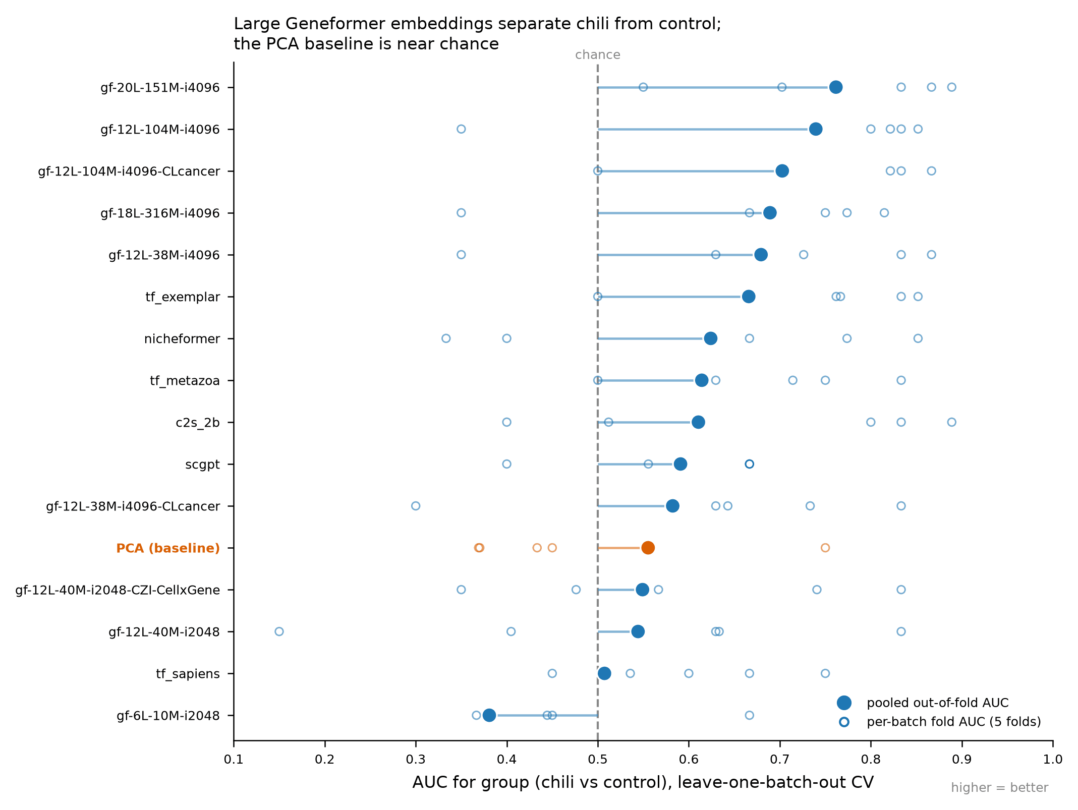
The five 4096-context Geneformer variants take the top five slots, beating the PCA baseline. Other models such as Transcriptformer, nicheformer, C2S or scGPT also beat the PCA baseline. Some models such as the smallest geneformer gf-6L-10M-i2048 lands below the baseline and below chance.
Batch 2 is the hardest fold for nearly every representation (0.15 to 0.55); It's large batch effects are partially reduced by some of the top scoring models such as the top scoring gf-20L-151M-i4096. Although single-cell Foundation Models have not been explicitly trained for batch correction, they can natively integrate batches better than traditional methods by focusing their variation into the relevant biological signal.
5Read genes off the winning embedding
Once a representation is chosen on a cross-validated criterion, the same UMAP can be recoloured by any gene: a candidate of your own, or the markers the source publication reports.
Example prompt:
Can you take embeddings for the best model and plot 2 umaps side by side - one coloured with log normalised expression of IL1R2 and another one coloured by group?
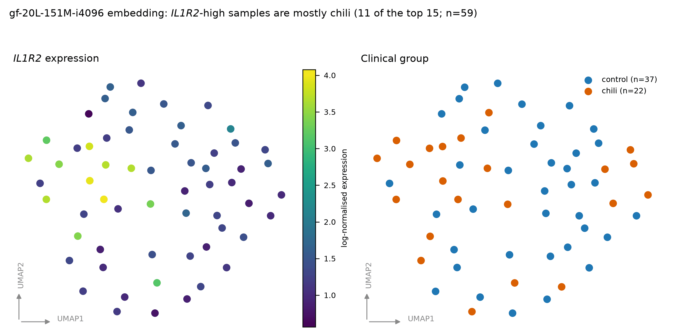
Expression is log-normalised from the raw counts, independently of the matrix used for PCA, and points are drawn low-to-high so high expressors are not hidden. The colourings agree on the left of the embedding: 11 of the 15 samples in the top IL1R2 quartile are ChILI, and the group medians are 2.37 against 1.27. Several ChILI samples on the right are IL1R2-low: what an AUC of 0.76 looks like, rather than a separated space. No differential-expression test was run.
Example prompt:
Get all the post-treatment biomarkers mentioned in this paper and plot their expression in the umap (one umap per biomarker). Add one extra umap at the beginning that is coloured by group (blue, white).
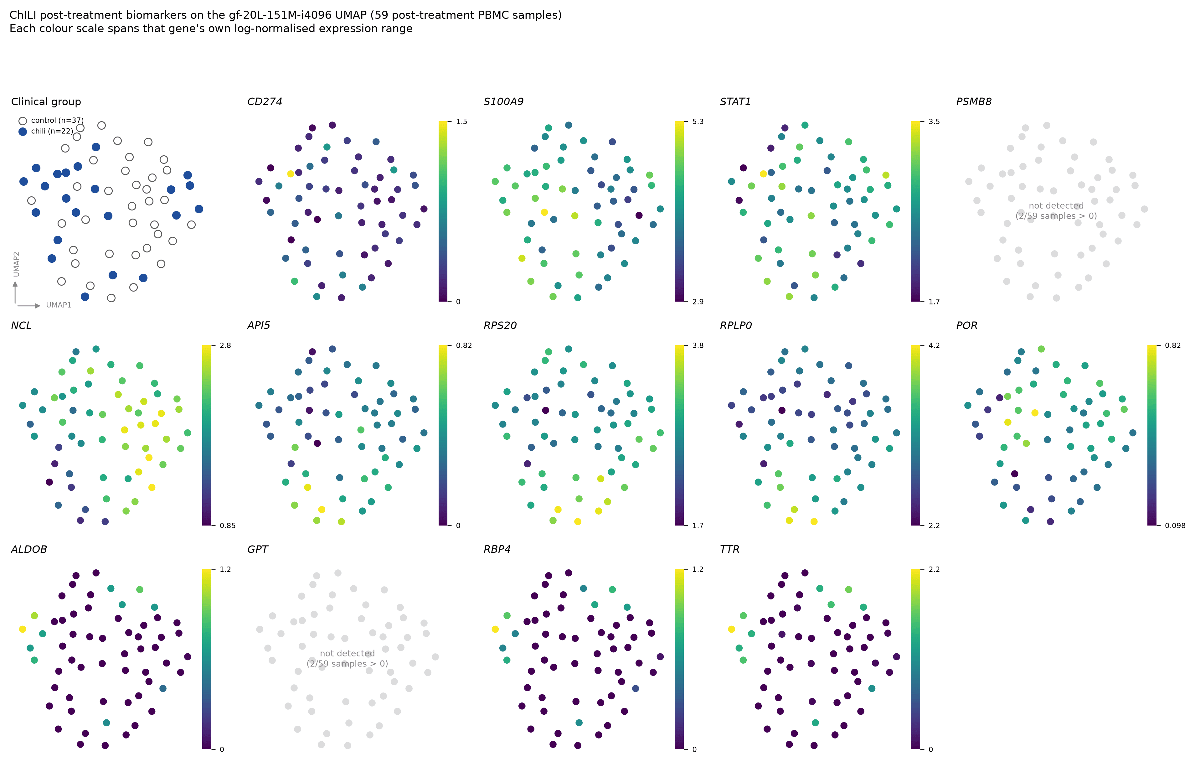
The paper names 16 post-treatment biomarkers, and the ones in the gene panel are plotted above. Some follow the same trend as the clinical group and some the opposite. A deeper analysis of how expression correlates with the embedding can help scientists further prioritise and validate biomarkers.
Takeaways
- Use these models to explore bulk RNA-seq samples, not only single cells.
- Use the embeddings to predict clinical outcomes, such as liver injury after immune checkpoint inhibitor treatment.
- Embed with the whole catalogue when the cohort is small. At these prices, model pre-selection is not worth the reasoning it costs.
- Always add a conventional baseline such as PCA. PCA on the same counts had near random predictions (0.55 AUC), while some of the larger bioFM models showed promising performance (0.76 AUC), the number the foundation models have to beat, and five of the 15 did not.
- Cross-validate on the technical grouping, not at random, and report the fold spread. This is key to ensure models can overcome batching effects and robustly capture biological signal.
Artifacts
| File | Contents |
|---|---|
post_treatment_adata_allmodels_pca.h5ad | the cohort with 16 representations and their UMAP coordinates in .obsm |
post_treatment_embeddings_pca.npz | the same matrices as plain arrays with obs_names |
post_treatment_embedding_manifest_pca.csv | per-model dimensions, dag_run_id, artifact_id, NaN counts |
umap_explorer_allmodels_pca.html | interactive 4 × 4 UMAP grid, 13 colour-by options |
logreg_group_auc_by_model.csv | pooled and per-batch AUCs for all 16 representations |
logreg_group_oof_predictions.csv | per-sample out-of-fold probabilities, with group and batch |
References
- Ji C, Kumpf S, Qian J, et al. Transcriptomic and proteomic characterization of cell and protein biomarkers of checkpoint inhibitor-induced liver injury. Cancer Immunology, Immunotherapy 2025;74:190. 10.1007/s00262-025-04033-z
- Trial registration: NCT04476563
- RNAseq data: GEO GSE287540, GSE287541
- Proteomic data: MassIVE MSV000096928