Recipe
Patient stratification with scFM embeddings
Single-cell foundation models produce one vector per cell. Clinical labels usually live one level higher: on the patient. To test whether a cell model has learned patient-level biology, we aggregate its cell embeddings without leaking patients across train and test folds, compare it with simple baselines, and check whether the result survives technical confounders.
In this cookbook, we use the Helical MCP to compute zero-shot scGPT and Geneformer-104M embeddings for tumour samples from the colorectal cancer atlas assembled by Chu et al.. We then average the cell embeddings within each patient and test whether they predict mismatch repair status, tumour side and grade. The analysis uses the Pelka cohort within the atlas: 25,228 cells from 127 tumour samples and 62 patients.
- Prepare the Pelka tumour samples from the colorectal atlas for Helical.
- Register them and get a quote for both models.
- Run the embeddings and download them.
- Plot cell-level UMAPs.
- Build patient representations and predict clinical labels.
- Localise the MMR signal by compartment.
- Check the unsupervised geometry.
See the full conversation. It takes 7 prompts and around 10 minutes. The steps below go through it one prompt at a time.
You need the Helical MCP connected (see Getting started) and around 1.3 credits.
1Get the data ready
The source dataset for this analysis is the integrated colorectal atlas published on Figshare. The full object contains 671,192 cells and 51,971 genes from 15 datasets. This analysis keeps Pelka.K tumour samples only, drops two samples with fewer than 100 tumour cells, and randomly samples up to 200 cells per sample.
The source X is log-normalised, so it cannot be sent directly to either model. prepare_crc_atlas.py reverses Seurat-style log normalisation. It uses nCount_RNA when that reconstructs integer counts and otherwise divides each cell by its smallest non-zero value, which recovers the UMI scale when at least one gene has a count of one.
Download the script from our public S3 bucket: aws s3 cp s3://helicalpackage/cookbooks/crc-patient-stratification-with-helical-mcp/prepare_crc_atlas.py . --no-sign-request
Example prompt:
Download the Chu et al. 2024 colorectal cancer atlas from figshare and get it ready for Helical. It's 671k cells from 15 studies. Only Pelka et al. 2021 has mismatch-repair (MMR) status, so keep Pelka tumour samples only, with 200 random cells per sample. Check which matrix holds raw counts, and tell me anything that looks off about the patient-level labels.
2Register and price
Example prompt:
Remove zero-only genes. Then register `pelka_crc_tumour_200.h5ad` and quote what it costs to embed with scGPT and Geneformer-104M. Don't start anything yet.
After upload, the platform reads the file back and confirms 25,228 cells and 29,509 genes. The quote uses each model's per-cell rate:
| Model | Credits per cell | Total |
|---|---|---|
| scGPT | 0.000018 | 0.45 |
| Geneformer-104M | 0.000033 | 0.83 |
| Both | 1.29 |
Nothing has run at this point, and no credits have been charged.
3Generate embeddings
Example prompt:
Go ahead - run both and download both embeddings when they're done. Check that each has 25,228 rows before using it.
Both embedding runs complete and pass validation.
The downloaded arrays contain one row per input cell, in the same order as the registered AnnData object:
| Model | Embedding shape |
|---|---|
| scGPT | 25,228 × 512 |
| Geneformer-104M | 25,228 × 768 |
The row-count check is important. A cell-level label from .obs is only valid for an embedding row if the order and number of cells still match.
4Visualise embeddings with UMAP
Example prompt:
Make cell-level UMAPs from each model's embeddings: cosine distance, 15 neighbours, same seed for both models. For each model, show four panels coloured by cell type (`ParentalCluster`), patient, MMR status and sort fraction. Then, for malignant cells only and for CD8 T cells only, make UMAPs coloured by patient and by MMR status. Tell me whether cells group by type, by patient or by MMR status, and whether this differs between scGPT and Geneformer.
We use the same UMAP settings for both models so the comparison is about the embeddings rather than plotting choices: cosine distance, 15 neighbours and random seed 42.
All cells
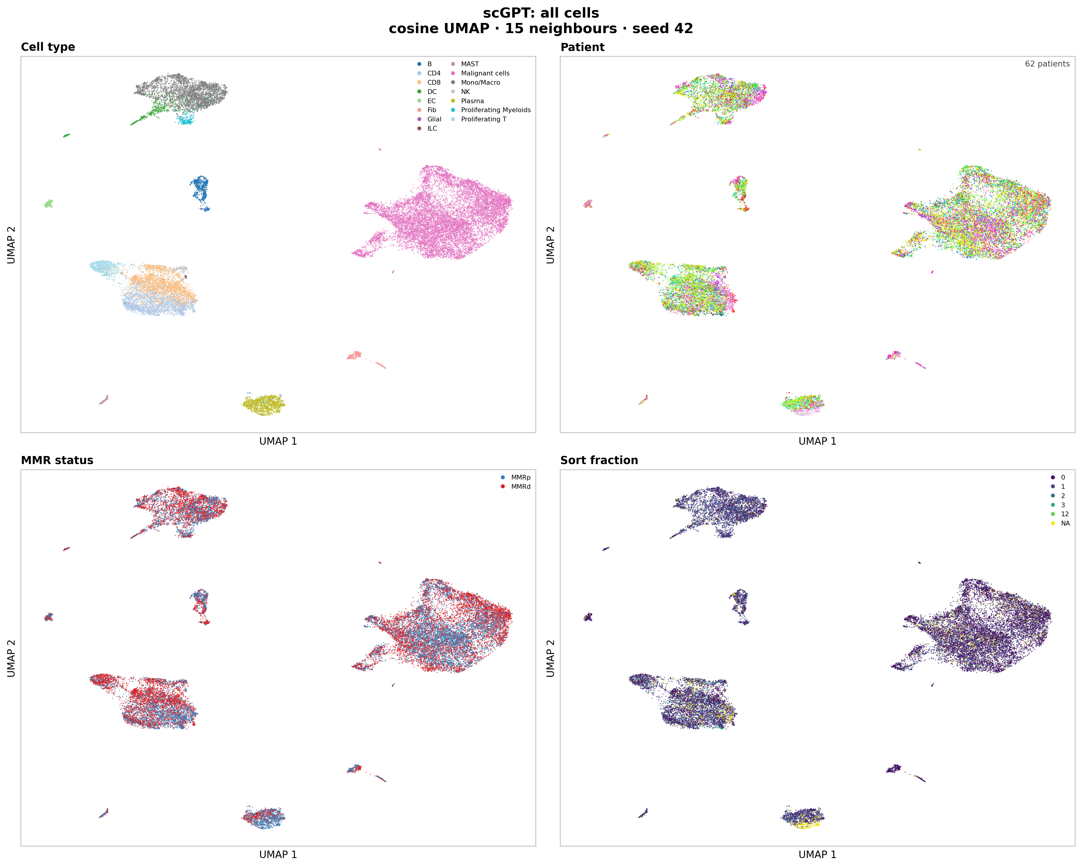
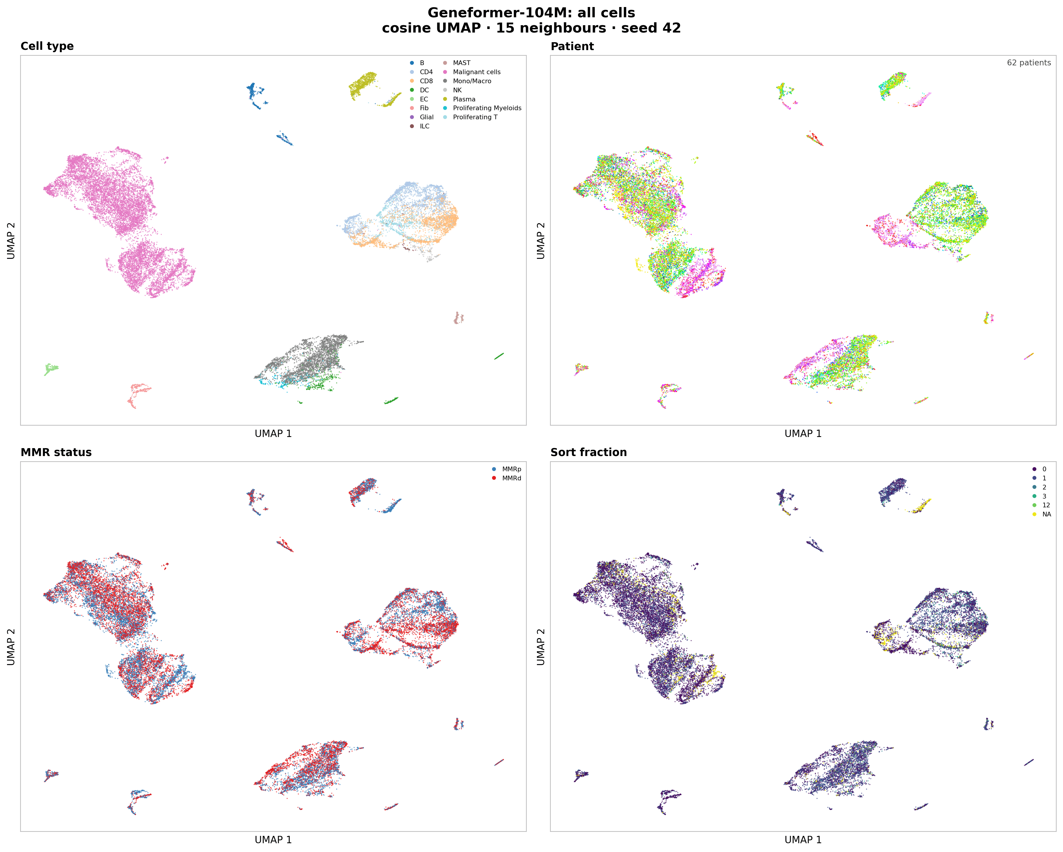
Both embeddings are dominated by cell type. A 15-neighbour enrichment score adjusted for label frequency is 0.91 for scGPT and 0.93 for Geneformer-104M across the 15 ParentalCluster classes.
Patient and MMR effects are present but weaker. Geneformer shows more local patient structure than scGPT (adjusted enrichment 0.28 versus 0.17) and more MMR structure (0.37 versus 0.26). Sort fraction is weaker still (0.24 versus 0.18). These are neighbourhood summaries, not classification scores, so they describe local geometry rather than predictive performance.
Malignant and CD8 cells
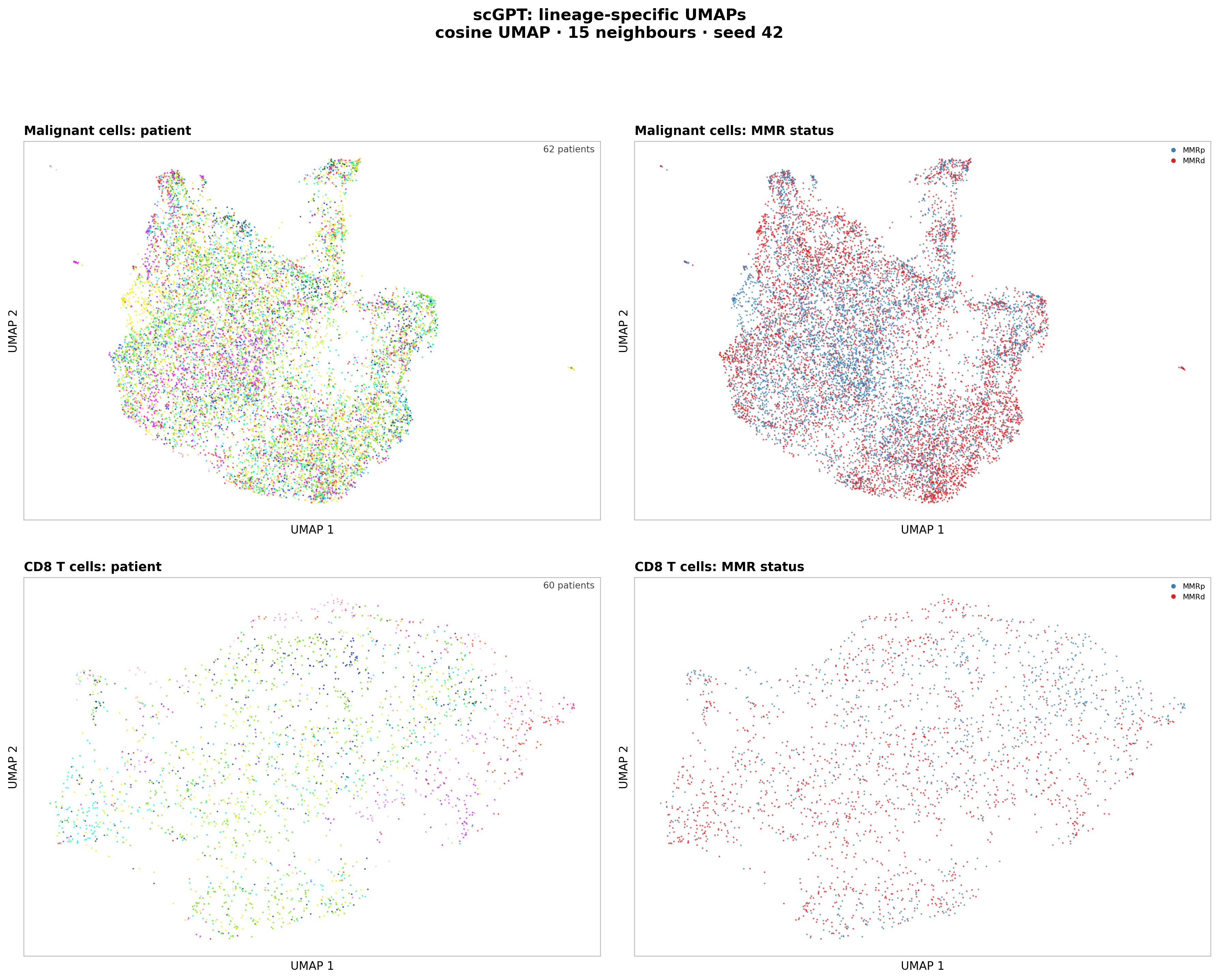
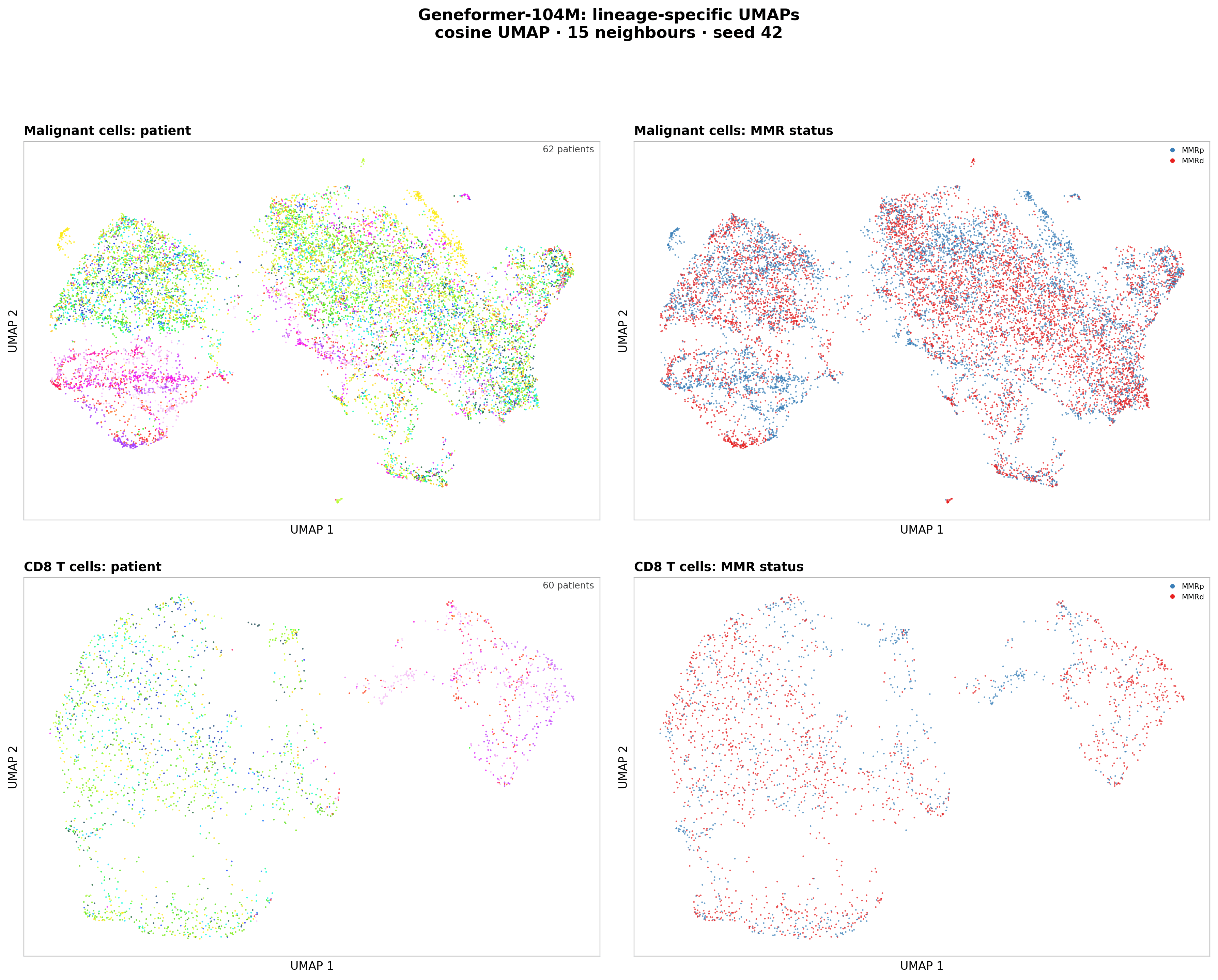
The lineage-restricted views tell the same story. Geneformer has stronger MMR neighbourhood enrichment in malignant cells (0.47 versus 0.30 for scGPT) and CD8 T cells (0.33 versus 0.23). Neither model produces two clean MMR islands.
5Build patient representations and predict clinical labels
We average all tumour-sample cell embeddings within each patient to create one 512-dimensional scGPT vector and one 768-dimensional Geneformer vector per patient. We add two model-free comparisons:
- Cell-type proportions from
ParentalCluster. - For MMR only, a metadata baseline containing tumour side and grade.
Example prompt:
Using the embeddings and the `.obs`, build one vector per patient by averaging all of the patient's tumour cells, for each model. There are 62 patients. Add two representations that need no model:

- cell-type proportions per patient, from `ParentalCluster`
- for MMR only, a metadata-only baseline using tumour side (`Site_patient`) and grade (`Grade_patient`)

For each representation, predict these patient-level labels with L2 logistic regression and repeated stratified 5-fold CV (10 repeats): MMR status (`MMRstatus_patient`), tumour side, and grade (high vs low, dropping the patient with grade "10"). Report AUROC with donor-bootstrap 95% CIs, in one table with labels as columns and representations as rows. Consider that with 62 patients, differences under about 0.05 are noise.
Every preprocessing step and classifier fit happens inside the cross-validation fold. Each patient receives ten out-of-fold probabilities, one from each repeat. Average those probabilities before calculating the headline AUROC, then bootstrap patients 10,000 times for the confidence interval.
| Representation | MMR status | Tumour side | Grade |
|---|---|---|---|
| scGPT mean embedding | 0.88 (0.79 to 0.96) | 0.71 (0.54 to 0.86) | 0.74 (0.55 to 0.90) |
| Geneformer-104M mean embedding | 0.94 (0.88 to 0.99) | 0.75 (0.61 to 0.87) | 0.60 (0.39 to 0.80) |
| Cell-type proportions | 0.81 (0.70 to 0.91) | 0.48 (0.26 to 0.71) | 0.71 (0.54 to 0.87) |
| Site + grade metadata | 0.58 (0.42 to 0.73) | Not evaluated | Not evaluated |
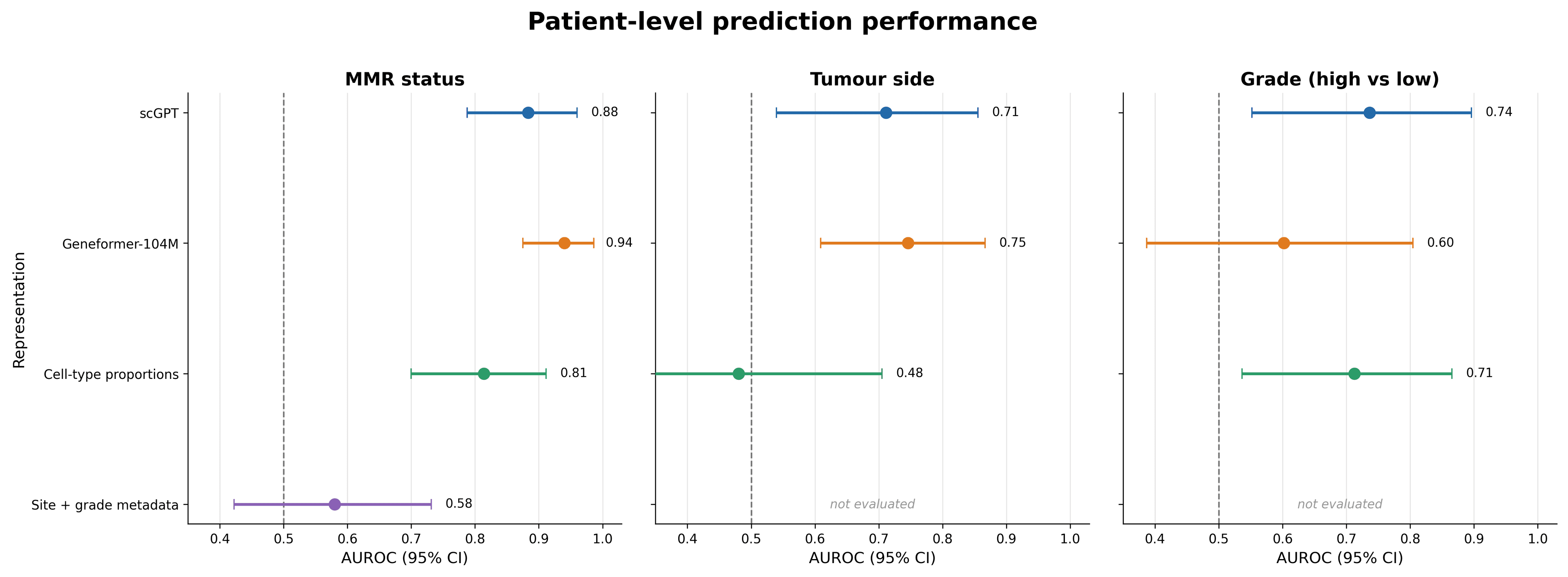
Geneformer embeddings are the strongest predictors of MMR status, although the confidence intervals overlap. For tumour side, the 0.04 model difference is not meaningful at this sample size. Grade is the least stable task: only 12 of the 61 evaluable patients are high grade, and all confidence intervals are broad.
Cell-type proportions reach 0.81 AUROC for MMR. Some patient-level MMR signal therefore comes from tumour microenvironment composition rather than cell state alone. The side-plus-grade baseline reaches only 0.58, so those two metadata fields do not explain the model result by themselves.
The out-of-fold probabilities show where the performance comes from. Geneformer places most MMRp patients near zero and most MMRd patients near one, but both models retain several confident errors. This is not a perfectly separable cohort.
6Localise the MMR signal by compartment
We repeat the MMR analysis after averaging embeddings from one compartment at a time, only keeping a patient when that compartment contains at least 20 cells.
Example prompt:
Repeat the MMR prediction using per-compartment patient vectors. Average only malignant cells (`ParentalCluster == "Malignant cells"`), then only T and NK cells (`CD4`, `CD8`, `Proliferating T`, `NK`, `ILC`), then only myeloid cells (`Mono/Macro`, `DC`, `Proliferating Myeloids`). Do it for both models. Drop patients with fewer than 20 cells in a compartment, and report how many patients were used each time. Then rerun the all-cells MMR prediction using only `sort_code == "0"` samples, to check that differences in sort fraction don't drive it.
| Compartment | Patients | scGPT AUROC | Geneformer-104M AUROC |
|---|---|---|---|
| All tumour-sample cells | 62 | 0.88 (0.79 to 0.96) | 0.94 (0.88 to 0.99) |
| Malignant cells | 62 | 0.89 (0.80 to 0.96) | 0.94 (0.86 to 0.99) |
| T and NK cells | 55 | 0.84 (0.72 to 0.93) | 0.90 (0.81 to 0.97) |
| Myeloid cells | 51 | 0.81 (0.67 to 0.92) | 0.85 (0.72 to 0.95) |
| All cells, sort code 0 only | 58 | 0.83 (0.71 to 0.93) | 0.90 (0.81 to 0.97) |
The malignant compartment preserves essentially all of the MMR signal. T and NK and myeloid compartments remain predictive, but their smaller cohorts and lower AUROCs make the evidence weaker. Geneformer remains ahead in every compartment.
Restricting the input to sort-code-0 samples lowers AUROC by 0.05 and 0.04 for scGPT and Geneformer respectively. The MMR signal remains strong, so sort fraction does not appear to be its main driver. This is a sensitivity analysis, not proof that every technical effect has been removed.
7Check unsupervised geometry
A high supervised AUROC does not mean that MMR status is the largest source of variation in the embedding. We check this directly with cosine-similarity heatmaps, hierarchical clustering and two-dimensional PCA.
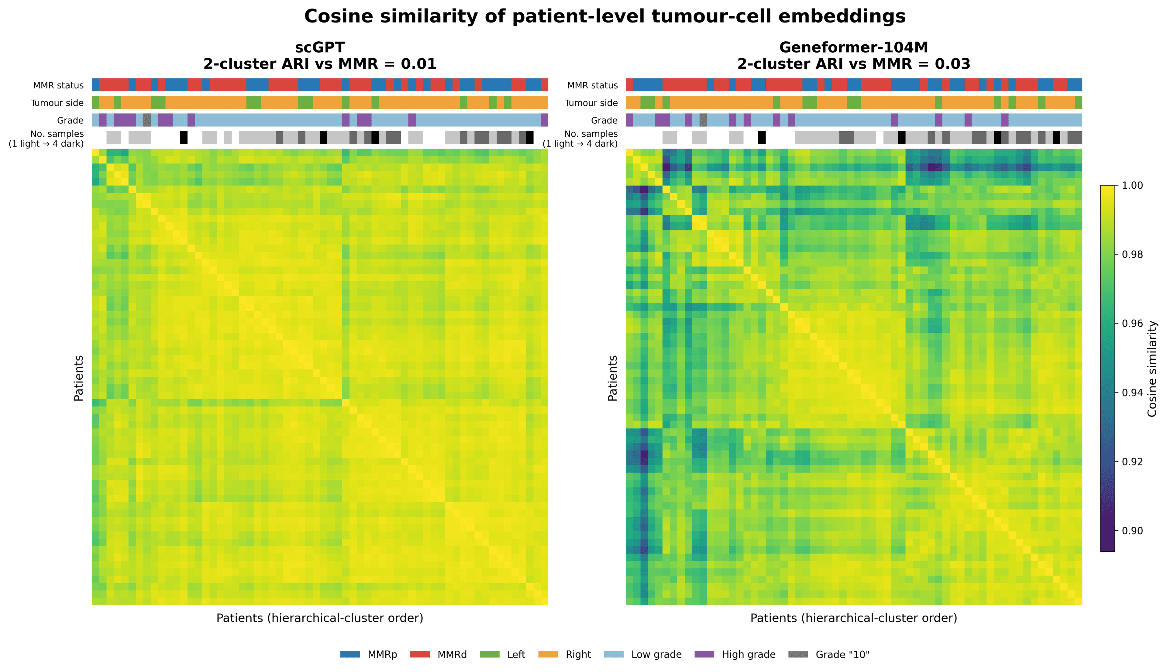
Average-linkage clustering on cosine distance produces an adjusted Rand index of 0.007 for scGPT and 0.026 for Geneformer when the top split is forced to two clusters and compared with MMR status. Both values are almost zero.
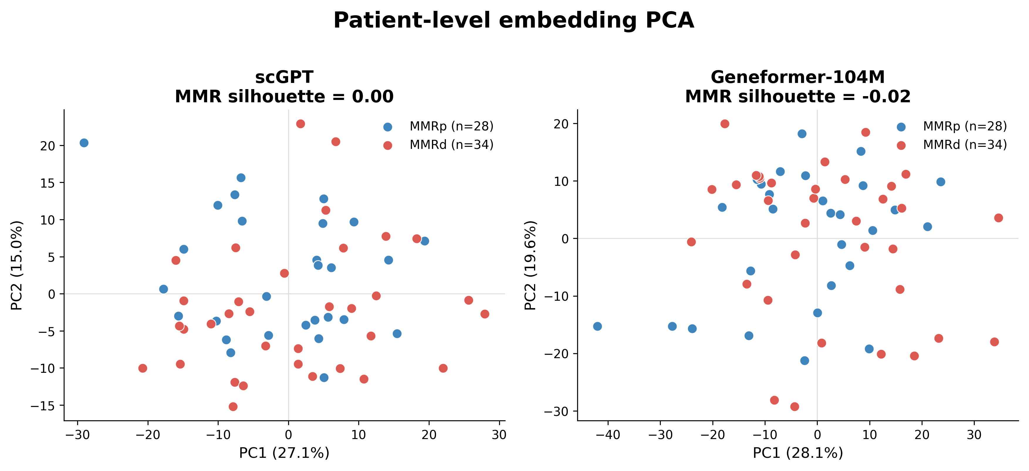
The MMR silhouette score in the displayed, feature-standardised two-dimensional PCA is also near zero: 0.004 for scGPT and -0.017 for Geneformer-104M. MMR is therefore predictable from distributed directions in the patient vectors, but it is not the dominant axis of unsupervised patient variation.
Takeaways
- Both models preserve cell identity strongly. Geneformer shows more patient and MMR structure at the cell level.
- Patient-averaged Geneformer embeddings give the strongest MMR result: AUROC 0.94 versus 0.88 for scGPT and 0.81 for cell-type proportions.
- The MMR signal is strongest in malignant cells, but also remains detectable in immune compartments and survives restriction to sort-code-0 samples.
- The result is supervised. MMR status does not define the top hierarchical split or the first two principal components.
- With 62 patients, small differences are unstable. We treat differences below about 0.05 as noise and read every AUROC together with its confidence interval.
- Cohort structure still matters. Tumour side is imbalanced and associated with MMR, grade has only 12 high-grade patients, and the number of cells per patient ranges from 200 to 800.
- The Helical MCP handles model-specific preprocessing and GPU inference. The scientific work remains in defining the patient representation, choosing baselines, keeping patients out of their own test folds, and testing confounders.
References
- Chu X, Li X, Zhang Y, et al. Integrative single-cell analysis of human colorectal cancer reveals patient stratification with distinct immune evasion mechanisms. Nature Cancer 2024;5:1409–1426. 10.1038/s43018-024-00807-z
- Pelka K, Hofree M, Chen JH, et al. Spatially organized multicellular immune hubs in human colorectal cancer. Cell 2021;184:4734–4752.e20. 10.1016/j.cell.2021.08.003
- Dataset download link: https://figshare.com/articles/dataset/_b_Integrative_single-cell_analysis_of_human_colorectal_cancer_reveals_patient_stratification_with_distinct_immune_evasion_mechanisms_b_/25323397