Recipe
Finding spatial niches with Nicheformer
Tumours are not uniform. Tumour, immune and stromal cells form local neighbourhoods, or niches, and the same niche can recur across patients. Finding them usually means annotating cell types first, then mapping where they sit. Bio foundation models offer another route: embed every spot, group similar spots into states, then look at which states sit next to each other on the tissue.
Nicheformer is a bio foundation model trained on single-cell and spatial transcriptomics. Running it yourself means getting the weights, a GPU and the tokenisation it expects. The Helical MCP handles that part.
In this cookbook, you compute zero-shot Nicheformer embeddings for a non-small cell lung cancer (NSCLC) Visium study through the Helical MCP. You then use them to define spot states and spatial niches, map both back onto the tissue, and check whether they recur in patients held out from discovery. The data are 88,520 Visium spots from 40 slides: eight cancer patients with tumour and matched background tissue, and two healthy donors.
- Prepare the spatial data and register it with Helical.
- Run Nicheformer and download the embeddings.
- Discover spot states and spatial niches on six patients.
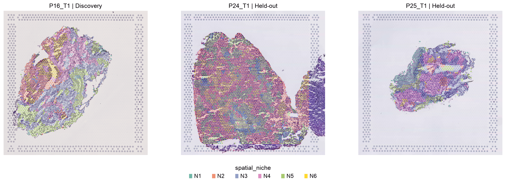
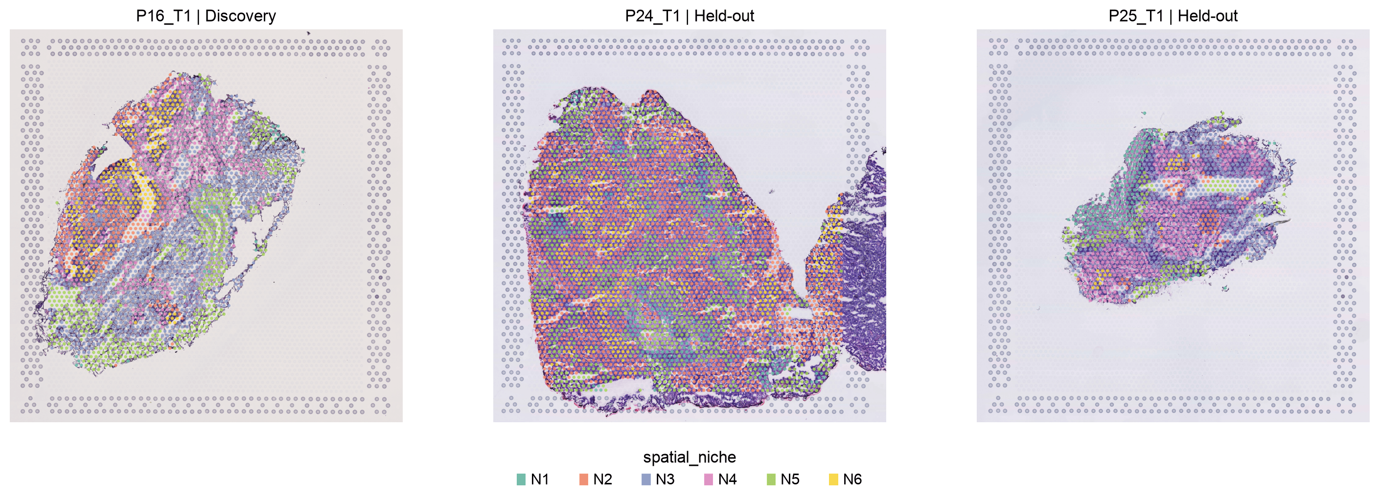
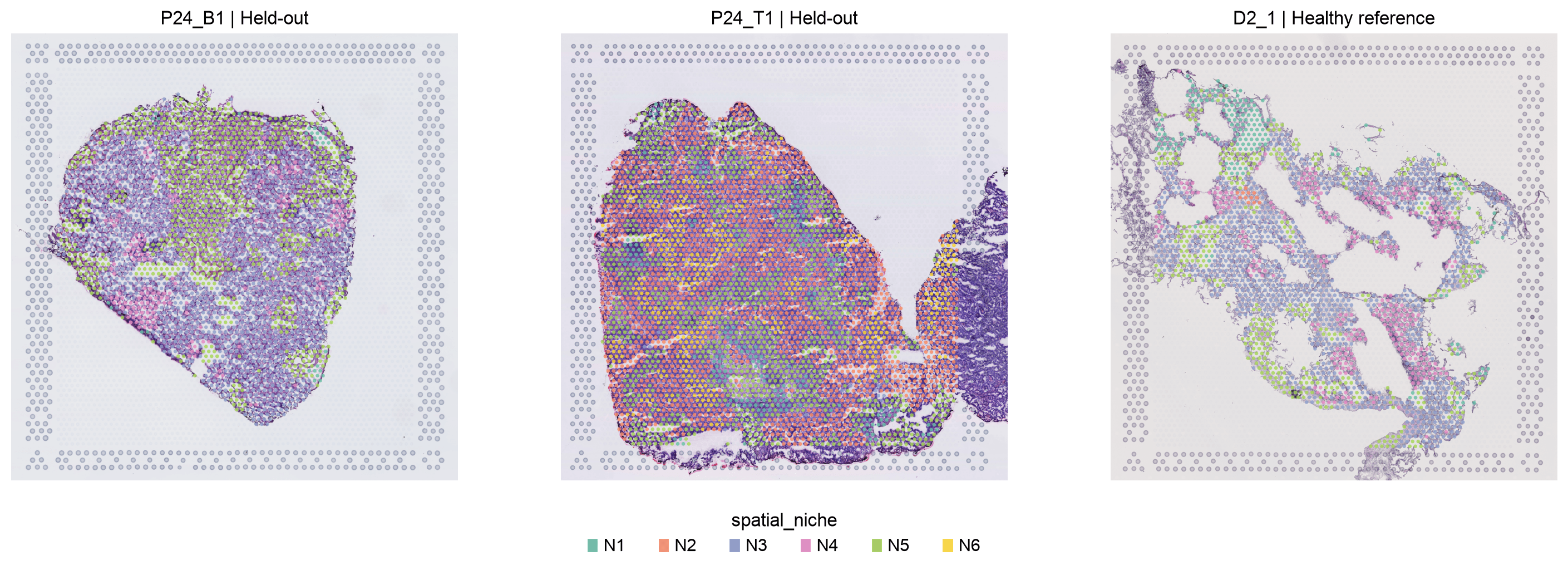
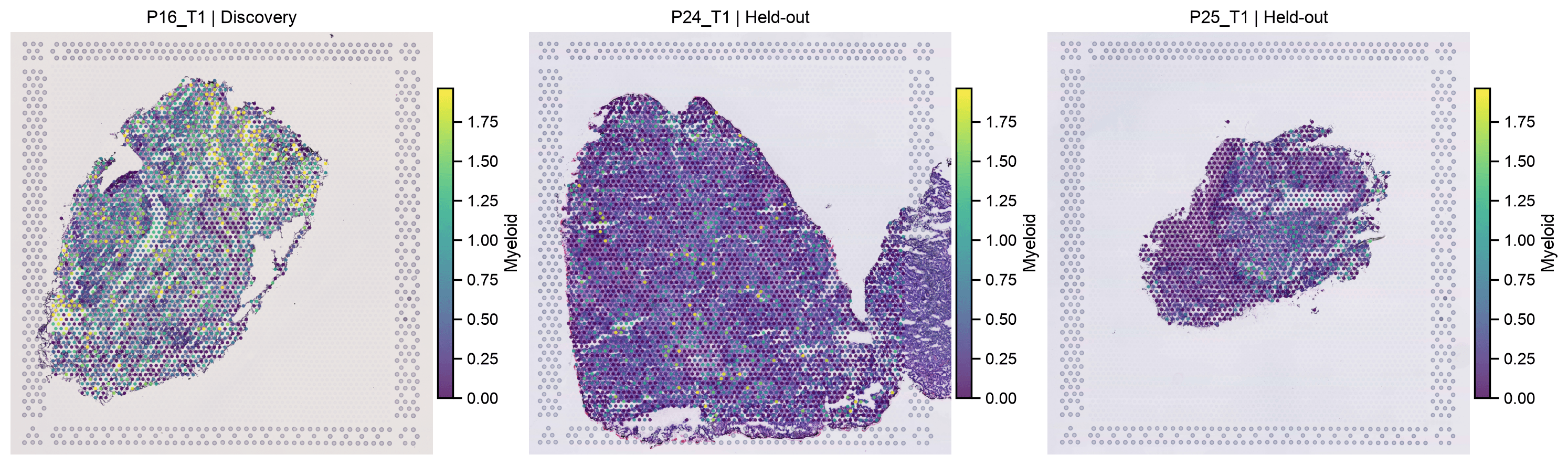
- Map them back onto the tissue.
- Check whether they recur in two held-out patients, against a QC-only baseline.
You need the Helical MCP connected (see Getting started) and about 2 credits.
1Set up the experiment
- Discovery patients: P10, P11, P15, P16, P17 and P19. States and niches are fitted on these.
- Held-out patients: P24 and P25. They are only used to test transfer.
- Healthy donors: D1 and D2, used as a descriptive comparison.
- Keep every slide from a patient on the same side of the split. Splitting spots at random would put the same patient on both sides.
- Fix these roles before looking at the embeddings.
from pathlib import Path
import json
import sys
import warnings
import importlib.metadata

import anndata as ad
import numpy as np
import pandas as pd
import scanpy as sc
import matplotlib.pyplot as plt
import seaborn as sns
from scipy import sparse
from sklearn.preprocessing import normalize
from IPython.display import display, Markdown
from IPython import get_ipython

get_ipython().run_line_magic('matplotlib', 'inline')

DATA_DIR = Path('data')
INPUT = DATA_DIR / 'nicheformer_input.h5ad'
IMAGES = DATA_DIR / 'spatial_images.h5ad'
EMBEDDING = DATA_DIR / 'nicheformer.npy'
OUTPUT = Path('results')
OUTPUT.mkdir(parents=True, exist_ok=True)
SEED = 42
DEVELOPMENT = ['P10', 'P11', 'P15', 'P16', 'P17', 'P19']
HOLDOUT = ['P24', 'P25']
sc.settings.n_jobs = 8
sc.settings.set_figure_params(dpi=100, frameon=False)
sns.set_context('notebook')
print('Python:', sys.version.split()[0])
print({name: importlib.metadata.version(name) for name in
       ['anndata', 'scanpy', 'numpy', 'pandas', 'scikit-learn']})
Python: 3.14.8
{'anndata': '0.13.4', 'scanpy': '1.12.4', 'numpy': '2.5.3', 'pandas': '3.0.6', 'scikit-learn': '1.9.1'}2Prepare the input
- The source
.Xholds raw UMI counts, which is what Nicheformer expects. Don't log-normalise or select genes before inference. - Keep the original spot order, IDs and coordinates. Map gene symbols back to the original 10x Ensembl IDs.
- Leave the tissue images out of the upload. They're kept in a separate file for plotting.
- Set the metadata to human, spatial, Visium. Helical's Nicheformer adapter has no dedicated Visium token, so the unknown-assay fallback is used.
- Visium spots mix several cells, while Nicheformer was trained on single cells. Treat this as an exploratory transfer across technologies. Example prompt:
Prepare the E-MTAB-13530 Visium slides for Nicheformer. Keep the raw counts in X, the original spot order, IDs and coordinates, and map gene symbols back to the original Ensembl IDs. Drop the tissue images and set the metadata to human, spatial, Visium. Tell me if anything looks off.
- The prepared input and the slide images are on our public S3 bucket. Download both into
data/to skip this step:
aws s3 cp s3://helicalpackage/cookbooks/spatial-demo/nicheformer_input.h5ad data/ --no-sign-request
aws s3 cp s3://helicalpackage/cookbooks/spatial-demo/spatial_images.h5ad data/ --no-sign-request
data = ad.read_h5ad(INPUT)
assert data.obs_names.is_unique, 'Repeated spot IDs break the alignment with the embeddings.'
print(f'{data.n_obs:,} spots × {data.n_vars:,} genes; '
      f'{data.obs["sample_id"].nunique()} slides from {data.obs["patient_id"].nunique()} subjects.')
88,520 spots × 36,601 genes; 40 slides from 10 subjects.
3Register, embed and download
3a. Register the dataset
Example prompt:
Register data/nicheformer_input.h5ad with Helical as E-MTAB-13530_Visium_spatial_demo. The observations are Visium spots; use patient_id as the donor column.
- Check the counts the platform returns: 88,520 spots and 36,601 genes.
3b. Run Nicheformer
Example prompt:
Generate embeddings for E-MTAB-13530_Visium_spatial_demo with the pretrained nicheformer model. Quote me the cost before starting the run.
- Review and approve the run when prompted. The recorded run was quoted at 1.77 credits.
- Nicheformer only sees expression. Tumour labels, patient IDs, images and coordinates are not inputs.
3c. Download the embeddings
Example prompt:
When the run succeeds, download the Nicheformer embeddings to data/nicheformer.npy.
4Attach the embeddings to the spots
- The
.npyfile has no spot IDs, so the rows line up because Helical keeps the input order. Check the row count before attaching the matrix.
embedding = np.load(EMBEDDING, allow_pickle=False)
assert embedding.ndim == 2 and embedding.shape[0] == data.n_obs, 'One embedding row per input spot is required.'
assert np.isfinite(embedding).all() and (np.linalg.norm(embedding, axis=1) > 0).all()
data.obsm['X_nicheformer'] = embedding.astype(np.float32)
data.obs['patient_id'] = data.obs['sample_id'].astype(str).str.split('_').str[0]
data.obs['tissue_group'] = data.obs['tissue_type'].astype(str).map(
    {'tumour': 'Tumour', 'border': 'Background', 'healthy': 'Healthy'})
assert data.obs['tissue_group'].notna().all()
data.obs['split'] = np.select(
    [data.obs['patient_id'].isin(DEVELOPMENT), data.obs['patient_id'].isin(HOLDOUT)],
    ['Discovery', 'Held-out'], default='Healthy reference')
print(f'Attached {embedding.shape[0]:,} spots × {embedding.shape[1]} embedding dimensions.')
Attached 88,520 spots × 512 embedding dimensions.
4a. Check the study design and technical covariates
- The source calls background tissue
border. In the original study, this is non-involved lung, not a tumour-boundary annotation. - Tissue labels are per slide: a tumour slide contains both tumour and its microenvironment.
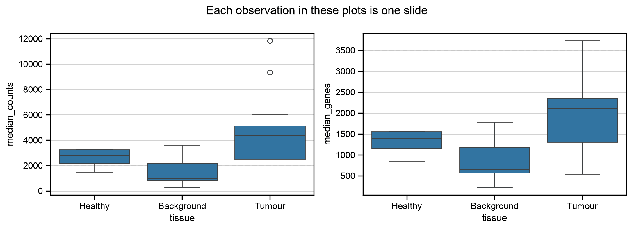
- Compute depth, detected genes and mitochondrial fraction, so you can check later whether structure follows technical variation.
symbols = data.var['gene_symbols'].astype(str)
data.var['mt'] = symbols.str.upper().str.startswith('MT-').to_numpy()
sc.pp.calculate_qc_metrics(data, qc_vars=['mt'], percent_top=None, log1p=False, inplace=True)
data.obs['log1p_total_counts'] = np.log1p(data.obs['total_counts'])
slide_table = data.obs.groupby('sample_id', observed=True).agg(
    patient=('patient_id', 'first'), tissue=('tissue_group', 'first'),
    split=('split', 'first'), spots=('patient_id', 'size'),
    median_counts=('total_counts', 'median'), median_genes=('n_genes_by_counts', 'median'))
display(slide_table)
display(pd.crosstab(slide_table['patient'], slide_table['tissue']))
fig, axes = plt.subplots(1, 2, figsize=(11, 4))
sns.boxplot(data=slide_table, x='tissue', y='median_counts', ax=axes[0])
sns.boxplot(data=slide_table, x='tissue', y='median_genes', ax=axes[1])
fig.suptitle('Each observation in these plots is one slide')
plt.tight_layout(); plt.show()
patient tissue split spots median_counts \
sample_id
D1_1 D1 Healthy Healthy reference 278 1478.5
D1_2 D1 Healthy Healthy reference 333 2391.0
D2_1 D2 Healthy Healthy reference 1852 3288.0
D2_2 D2 Healthy Healthy reference 2432 3231.5
P10_B1 P10 Background Discovery 1755 989.0
P10_B2 P10 Background Discovery 1842 597.0
P10_T1 P10 Tumour Discovery 2200 4434.0
P10_T2 P10 Tumour Discovery 1986 4951.0
P10_T3 P10 Tumour Discovery 2610 4182.0
P10_T4 P10 Tumour Discovery 2479 2393.0
P11_B1 P11 Background Discovery 2873 1442.0
P11_B2 P11 Background Discovery 2846 856.0
P11_T1 P11 Tumour Discovery 1110 1822.5
P11_T2 P11 Tumour Discovery 1176 2053.0
P11_T3 P11 Tumour Discovery 1735 953.0
P11_T4 P11 Tumour Discovery 1811 868.0
P15_B1 P15 Background Discovery 2844 3035.5
P15_B2 P15 Background Discovery 2824 3626.5
P15_T1 P15 Tumour Discovery 2624 5977.5
P15_T2 P15 Tumour Discovery 3131 4833.0
P16_B1 P16 Background Discovery 3123 514.0
P16_B2 P16 Background Discovery 3351 263.0
P16_T1 P16 Tumour Discovery 2262 4333.0
P16_T2 P16 Tumour Discovery 2210 4080.5
P17_B1 P17 Background Discovery 1522 921.5
P17_B2 P17 Background Discovery 1093 986.0
P17_T1 P17 Tumour Discovery 2658 11850.0
P17_T2 P17 Tumour Discovery 2953 9334.0
P19_B1 P19 Background Discovery 2197 651.0
P19_B2 P19 Background Discovery 2120 941.5
P19_T1 P19 Tumour Discovery 2512 6045.5
P19_T2 P19 Tumour Discovery 2369 5055.0
P24_B1 P24 Background Held-out 2581 2751.0
P24_B2 P24 Background Held-out 3019 2030.0
P24_T1 P24 Tumour Held-out 3426 3342.0
P24_T2 P24 Tumour Held-out 3491 2561.0
P25_B1 P25 Background Held-out 1965 2158.0
P25_B2 P25 Background Held-out 2161 2325.0
P25_T1 P25 Tumour Held-out 1308 5005.5
P25_T2 P25 Tumour Held-out 1458 5390.0
median_genes
sample_id
D1_1 852.0
D1_2 1247.0
D2_1 1554.0
D2_2 1566.0
P10_B1 654.0
P10_B2 438.5
P10_T1 2192.0
P10_T2 2350.5
P10_T3 2047.5
P10_T4 1312.0
P11_B1 927.0
P11_B2 604.0
P11_T1 1033.5
P11_T2 1141.0
P11_T3 608.0
P11_T4 538.0
P15_B1 1507.5
P15_B2 1786.0
P15_T1 2544.0
P15_T2 2183.0
P16_B1 390.0
P16_B2 218.0
P16_T1 1959.5
P16_T2 1914.5
P17_B1 591.0
P17_B2 604.0
P17_T1 3731.0
P17_T2 3333.0
P19_B1 486.0
P19_B2 649.5
P19_T1 2654.5
P19_T2 2328.0
P24_B1 1422.0
P24_B2 1161.0
P24_T1 1507.0
P24_T2 1276.0
P25_B1 1165.0
P25_B2 1247.0
P25_T1 2333.5
P25_T2 2389.5 tissue Background Healthy Tumour patient D1 0 2 0 D2 0 2 0 P10 2 0 4 P11 2 0 4 P15 2 0 2 P16 2 0 2 P17 2 0 2 P19 2 0 2 P24 2 0 2 P25 2 0 2
5Discover spot states, then spatial niches
- Normalise each embedding to unit length.
- Fit eight spot states on a slide-balanced sample from the discovery patients, then assign every other spot to its nearest state.
- Describe each spot's neighbourhood by the states of up to six physical neighbours on the same slide, including itself.
- Fit six niches on these neighbourhood profiles from discovery patients, then transfer them unchanged.
- Eight states and six niches are fixed demo settings, not estimates of the true number of populations.
- Spots with no neighbours are flagged as isolated.
from sklearn.cluster import KMeans

N_STATES, N_NICHES, PER_SLIDE = 8, 6, 1000
HEX_OFFSETS = [(0, 2), (0, -2), (1, 1), (1, -1), (-1, 1), (-1, -1)]


def balanced_sample(mask, obs, per_slide, rng):
    '''Up to `per_slide` spots from every slide in `mask`, so large sections don't dominate.'''
    index = np.flatnonzero(mask)
    slides = obs['sample_id'].astype(str).to_numpy()[index]
    return np.concatenate([rng.choice(group, min(per_slide, len(group)), replace=False)
                           for _, group in pd.Series(index).groupby(slides)])


def visium_adjacency(obs):
    '''Physical neighbours on the Visium hexagonal grid, within each slide.'''
    spots = pd.DataFrame({'slide': obs['sample_id'].astype(str).to_numpy(),
                          'row': obs['array_row'].to_numpy(), 'col': obs['array_col'].to_numpy(),
                          'i': np.arange(len(obs))})
    edges = []
    for d_row, d_col in HEX_OFFSETS:
        shifted = spots.assign(row=spots['row'] + d_row, col=spots['col'] + d_col)
        pairs = shifted.merge(spots, on=['slide', 'row', 'col'], suffixes=('', '_neighbour'))
        edges.append(pairs[['i', 'i_neighbour']].to_numpy())
    edges = np.concatenate(edges)
    return sparse.csr_matrix((np.ones(len(edges)), (edges[:, 0], edges[:, 1])),
                             shape=(len(obs), len(obs)))


def fit_spatial_states_and_niches(embedding, obs, development_patients, random_state):
    rng = np.random.default_rng(random_state)
    x = normalize(embedding)
    fit_index = balanced_sample(obs['patient_id'].isin(development_patients).to_numpy(), obs, PER_SLIDE, rng)

    state_model = KMeans(N_STATES, n_init=10, random_state=random_state).fit(x[fit_index])
    state_dist = state_model.transform(x)
    state_codes = state_dist.argmin(axis=1)
    state_distance = state_dist.min(axis=1)
    state_in_reference = state_distance <= np.quantile(state_distance[fit_index], 0.95)

    adjacency = visium_adjacency(obs)
    one_hot = np.eye(N_STATES)[state_codes]
    with_self = adjacency + sparse.identity(len(obs), format='csr')
    proportions = np.asarray(with_self @ one_hot)
    proportions /= proportions.sum(axis=1, keepdims=True)

    niche_model = KMeans(N_NICHES, n_init=10, random_state=random_state).fit(proportions[fit_index])
    niche_dist = niche_model.transform(proportions)
    niche_distance = niche_dist.min(axis=1)
    niche_covered = niche_distance <= np.quantile(niche_distance[fit_index], 0.95)

    state_names = [f'S{k + 1}' for k in range(N_STATES)]
    niche_names = [f'N{k + 1}' for k in range(N_NICHES)]
    assignments = pd.DataFrame({
        'niche_covered': niche_covered,
        'qc_pass': (obs['total_counts'].to_numpy() >= 500) & (obs['n_genes_by_counts'].to_numpy() >= 200),
        'n_neighbors': np.asarray(adjacency.sum(axis=1)).ravel().astype(int),
    }, index=obs.index)
    coverage = pd.DataFrame({'patient_id': obs['patient_id'].to_numpy(), 'split': obs['split'].to_numpy(),
                             'state_in_reference': state_in_reference, 'niche_covered': niche_covered})
    coverage = coverage.groupby(['patient_id', 'split'], observed=True).agg(
        spots=('state_in_reference', 'size'), state_coverage=('state_in_reference', 'mean'),
        niche_coverage=('niche_covered', 'mean')).reset_index()
    return {
        'states': np.array(state_names)[state_codes],
        'niches': np.array(niche_names)[niche_dist.argmin(axis=1)],
        'state_distance': state_distance, 'state_in_reference': state_in_reference,
        'assignments': assignments, 'neighborhood_proportions': proportions, 'adjacency': adjacency,
        'coverage': coverage,
        'niche_centroid_proportions': pd.DataFrame(niche_model.cluster_centers_, index=niche_names, columns=state_names),
        'models': {'states': state_model, 'niches': niche_model},
    }


discovery = fit_spatial_states_and_niches(
    data.obsm['X_nicheformer'], data.obs, development_patients=DEVELOPMENT, random_state=SEED,
)
data.obs['spot_state'] = pd.Categorical(discovery['states'])
data.obs['spatial_niche'] = pd.Categorical(discovery['niches'])
state_palette = dict(zip(data.obs['spot_state'].cat.categories, sns.color_palette('tab10', 8).as_hex()))
niche_palette = dict(zip(data.obs['spatial_niche'].cat.categories, sns.color_palette('Set2', 6).as_hex()))
data.uns['spot_state_colors'] = list(state_palette.values())
data.uns['spatial_niche_colors'] = list(niche_palette.values())
data.obs['state_distance'] = discovery['state_distance']
data.obs['state_in_reference'] = discovery['state_in_reference']
data.obs['niche_in_reference'] = discovery['assignments']['niche_covered'].to_numpy()
data.obs['qc_pass'] = discovery['assignments']['qc_pass'].to_numpy()
data.obs['spatial_degree'] = discovery['assignments']['n_neighbors'].to_numpy()
data.obs['isolated_spot'] = data.obs['spatial_degree'].eq(0)
data.obsm['state_neighborhood_proportions'] = discovery['neighborhood_proportions']
data.obsp['physical_neighbors'] = discovery['adjacency']
display(discovery['coverage'])
display(discovery['niche_centroid_proportions'].round(3))
display(data.obs.groupby('spot_state', observed=True).agg(
    spots=('sample_id', 'size'), qc_pass_fraction=('qc_pass', 'mean'),
    median_counts=('total_counts', 'median'), median_genes=('n_genes_by_counts', 'median')))
print('QC flag for sensitivity analysis: at least 500 UMIs and 200 detected genes; no rows dropped from the embedding.')
print(f'Isolated spots with self-only composition: {data.obs["isolated_spot"].sum():,}')
patient_id split spots state_coverage niche_coverage 0 D1 Healthy reference 611 0.900164 0.859247 1 D2 Healthy reference 4284 0.934641 0.984360 2 P10 Discovery 12872 0.952921 0.964108 3 P11 Discovery 11551 0.941304 0.937927 4 P15 Discovery 11423 0.954653 0.982404 5 P16 Discovery 10946 0.967020 0.854193 6 P17 Discovery 8226 0.968271 0.986263 7 P19 Discovery 9198 0.939335 0.958143 8 P24 Held-out 12517 0.863466 0.978429 9 P25 Held-out 6892 0.960389 0.976204
       S1     S2     S3     S4     S5     S6     S7     S8
N1  0.002  0.256  0.122  0.000  0.001  0.030  0.010  0.579
N2  0.715  0.001  0.019  0.108  0.035  0.101  0.017  0.004
N3  0.011  0.001  0.039  0.001  0.137  0.191  0.611  0.009
N4  0.013  0.000  0.004  0.012  0.760  0.027  0.182  0.001
N5  0.021  0.007  0.412  0.004  0.012  0.343  0.083  0.118
N6  0.122  0.001  0.003  0.823  0.035  0.012  0.004  0.001
            spots  qc_pass_fraction  median_counts  median_genes
spot_state
S1           8386          1.000000         5257.0        2264.0
S2           5239          0.000764          181.0         151.0
S3          12658          0.999842         1070.0         693.0
S4           5958          1.000000        12614.0        4155.0
S5          10370          1.000000         9716.0        3430.0
S6          15895          1.000000         1994.0        1126.0
S7          17492          1.000000         3916.5        1841.0
S8          12522          0.530187          515.0         376.0
QC flag for sensitivity analysis: at least 500 UMIs and 200 detected genes; no rows dropped from the embedding.
Isolated spots with self-only composition: 335
6View the embedding
- Colour the UMAP by tissue, patient and depth before reading the state colours. Patient-specific islands or depth gradients point to technical structure.
- The UMAP is only a view. It isn't used to fit states or niches.
sc.pp.neighbors(data, use_rep='X_nicheformer', n_neighbors=15,
                metric='cosine', random_state=SEED, key_added='nicheformer_neighbors')
sc.tl.umap(data, neighbors_key='nicheformer_neighbors', random_state=SEED)
sc.pl.umap(data, color=['tissue_group', 'patient_id', 'log1p_total_counts',
                       'spot_state', 'spatial_niche', 'split'], ncols=3,
           wspace=0.35, size=3, show=False)
plt.savefig(OUTPUT / 'embedding_umap.png', dpi=150, bbox_inches='tight')
plt.show()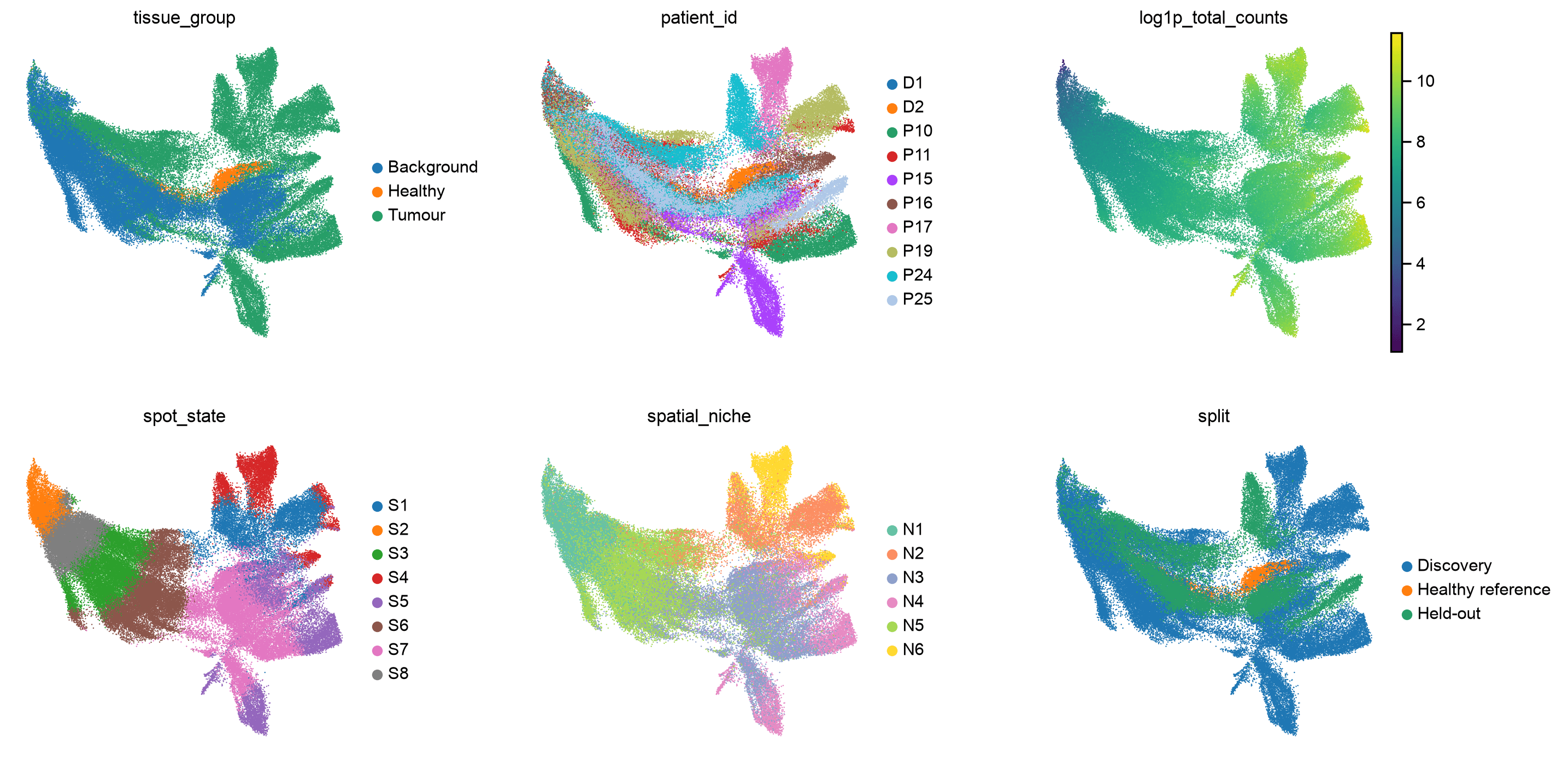
7Read the states with marker programs
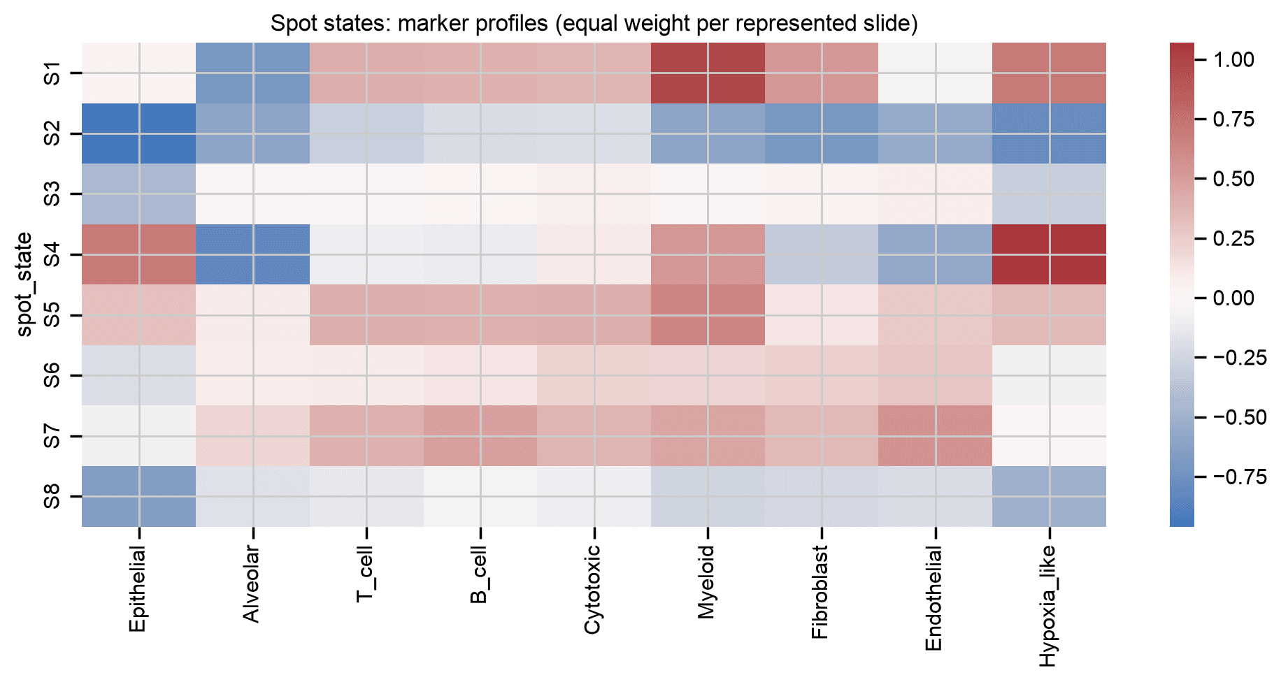
- Score nine marker programs per spot: mean log1p counts per 10,000 UMIs.
- The scores come from the same expression data as the embeddings, so they help interpretation but aren't independent validation.
- Epithelial markers also appear in normal epithelium, so an epithelial or hypoxia-like score alone doesn't mark tumour.
programs = {
    'Epithelial': ['EPCAM', 'KRT8', 'KRT18', 'KRT19'],
    'Alveolar': ['SFTPA1', 'SFTPB', 'SFTPC', 'SFTPD'],
    'T_cell': ['CD3D', 'CD3E', 'TRAC'],
    'B_cell': ['MS4A1', 'CD79A', 'CD79B'],
    'Cytotoxic': ['NKG7', 'GNLY', 'PRF1'],
    'Myeloid': ['LST1', 'TYROBP', 'FCER1G'],
    'Fibroblast': ['COL1A1', 'COL1A2', 'DCN'],
    'Endothelial': ['PECAM1', 'VWF', 'KDR'],
    'Hypoxia_like': ['CA9', 'SLC2A1', 'VEGFA', 'LDHA'],
}
marker_report = []
totals = data.obs['total_counts'].to_numpy()
for name, genes in programs.items():
    mask = symbols.isin(genes).to_numpy()
    present = symbols[mask].tolist()
    assert len(present) >= 2, (name, present)
    x = data.X[:, mask].astype(np.float32)
    x = sparse.diags(10000 / np.maximum(totals, 1)) @ x
    x.data = np.log1p(x.data)
    data.obs[f'score_{name}'] = np.asarray(x.mean(axis=1)).ravel()
    marker_report.append({'program': name, 'present': ', '.join(present),
                          'missing': ', '.join(sorted(set(genes) - set(present)))})
display(pd.DataFrame(marker_report))
score_cols = [f'score_{name}' for name in programs]
scores = data.obs[score_cols]
is_development = data.obs['patient_id'].isin(DEVELOPMENT)
z = (scores - scores.loc[is_development].mean()) / scores.loc[is_development].std().clip(lower=1e-6)
profile_frame = z.join(data.obs[['sample_id', 'patient_id', 'tissue_group', 'spot_state', 'spatial_niche', 'split']])
state_profiles = profile_frame.groupby(['sample_id', 'spot_state'], observed=True)[score_cols].mean()
state_profiles = state_profiles.groupby('spot_state', observed=True).mean()
fig, ax = plt.subplots(figsize=(10, 5))
sns.heatmap(state_profiles.rename(columns=lambda c: c.removeprefix('score_')),
            cmap='vlag', center=0, ax=ax)
ax.set_title('Spot states: marker profiles (equal weight per represented slide)')
plt.tight_layout(); plt.savefig(OUTPUT / 'state_markers.png', dpi=150); plt.show()
program present missing 0 Epithelial EPCAM, KRT8, KRT18, KRT19 1 Alveolar SFTPB, SFTPC, SFTPA1, SFTPD 2 T_cell CD3E, CD3D, TRAC 3 B_cell MS4A1, CD79B, CD79A 4 Cytotoxic GNLY, PRF1, NKG7 5 Myeloid FCER1G, LST1, TYROBP 6 Fibroblast COL1A2, DCN, COL1A1 7 Endothelial KDR, VWF, PECAM1 8 Hypoxia_like SLC2A1, VEGFA, CA9, LDHA
8Map states and niches onto the tissue
- Each slide's histology image is stored under its slide ID in
spatial_images.h5ad. - Compare a discovery patient (P16) with both held-out patients (P24 and P25). A colour means the same state or niche in every panel.
- Change the slide list to look at any of the 40 sections.
images = ad.read_h5ad(IMAGES)
assert set(images.uns['spatial']) == set(data.obs['sample_id'].astype(str)), 'Every slide needs its image.'
state_palette = dict(zip(data.obs['spot_state'].cat.categories, sns.color_palette('tab10', 8).as_hex()))
niche_palette = dict(zip(data.obs['spatial_niche'].cat.categories, sns.color_palette('Set2', 6).as_hex()))

def plot_slides(slides, colour, palette=None, vmin=None, vmax=None):
    from matplotlib.collections import PatchCollection
    from matplotlib.patches import Circle, Patch
    from matplotlib.colors import Normalize

    fig, axes = plt.subplots(1, len(slides), figsize=(5 * len(slides), 5), squeeze=False)
    for ax, slide_id in zip(axes.ravel(), slides):
        mask = data.obs['sample_id'].astype(str).eq(slide_id).to_numpy()
        bundle = images.uns['spatial'][slide_id]
        scale = bundle['scalefactors']['tissue_hires_scalef']
        radius = bundle['scalefactors']['spot_diameter_fullres'] * scale / 2
        xy = data.obsm['spatial'][mask] * scale
        patches = [Circle(point, radius) for point in xy]
        ax.imshow(bundle['images']['hires'], origin='upper')
        if palette is not None:
            colours = [palette[str(value)] for value in data.obs.loc[mask, colour]]
            collection = PatchCollection(patches, facecolors=colours, edgecolors='none', alpha=0.8)
        else:
            collection = PatchCollection(patches, cmap='viridis', norm=Normalize(vmin, vmax),
                                         edgecolors='none', alpha=0.8)
            collection.set_array(data.obs.loc[mask, colour].to_numpy(dtype=float))
            fig.colorbar(collection, ax=ax, fraction=0.035, pad=0.01, label=colour.removeprefix('score_'))
        ax.add_collection(collection)
        ax.set_title(f'{slide_id} | {data.obs.loc[mask, "split"].iloc[0]}')
        ax.set_aspect('equal'); ax.axis('off')
    if palette is not None:
        fig.legend(handles=[Patch(color=value, label=key) for key, value in palette.items()],
                   loc='lower center', ncol=len(palette), frameon=False, title=colour)
    fig.tight_layout(rect=(0, 0.12 if palette else 0, 1, 1))
    fig.savefig(OUTPUT / f'spatial_{colour}_{"_".join(slides)}.png', dpi=150, bbox_inches='tight')
    plt.show()

plot_slides(['P16_T1', 'P24_T1', 'P25_T1'], 'spot_state', state_palette)
plot_slides(['P16_T1', 'P24_T1', 'P25_T1'], 'spatial_niche', niche_palette)
plot_slides(['P24_B1', 'P24_T1', 'D2_1'], 'spatial_niche', niche_palette)
program = 'score_Myeloid'  # also try score_Fibroblast, score_T_cell or score_Epithelial
plot_slides(['P16_T1', 'P24_T1', 'P25_T1'], program,
            vmin=0, vmax=float(data.obs[program].quantile(0.98)))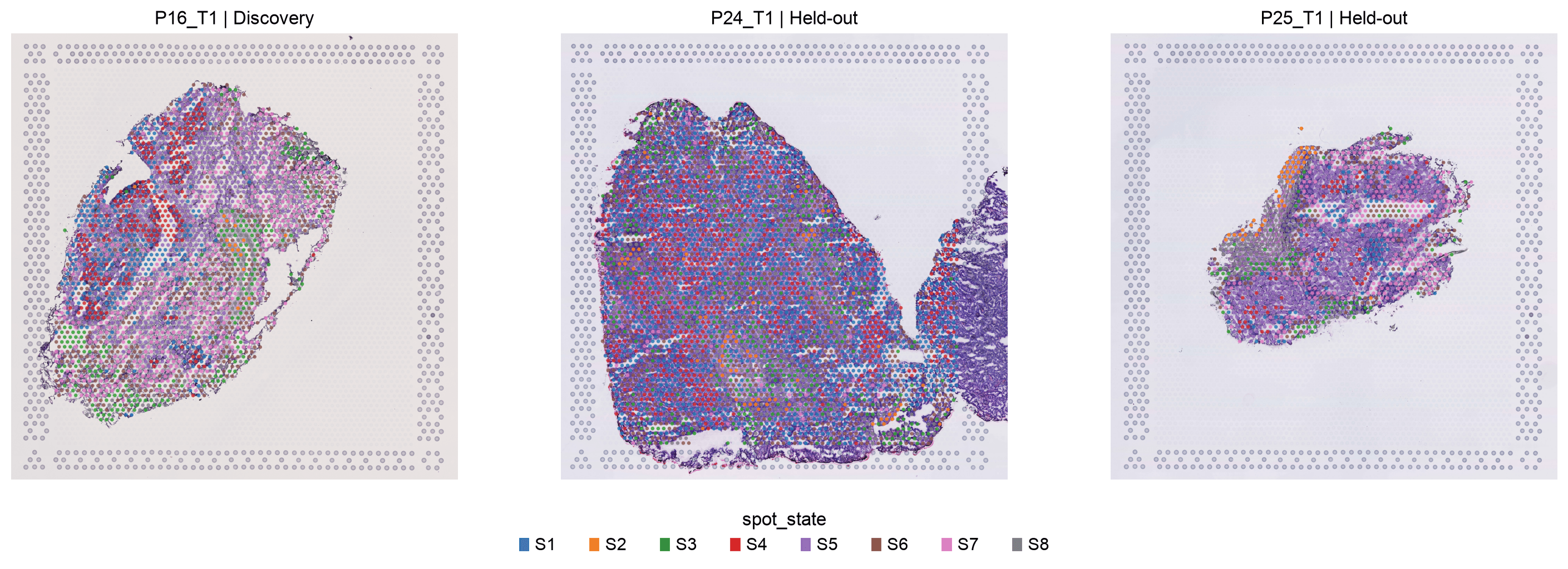
9Do the niches recur across patients?
- Compute niche fractions per patient and tissue, averaging slides so a large section doesn't dominate.
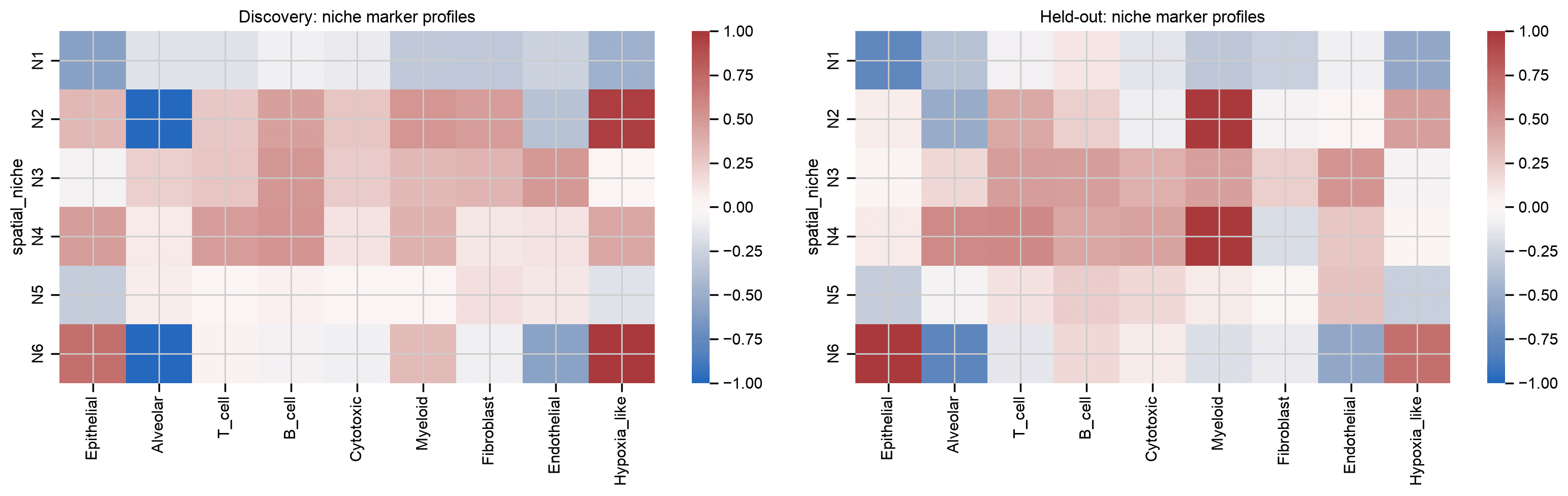
- Held-out patients didn't contribute to fitting, but every spot is assigned to its nearest niche, so recurrence alone isn't enough. Also compare reference coverage and marker profiles between discovery and held-out patients.
slide_fractions = pd.crosstab(data.obs['sample_id'], data.obs['spatial_niche'], normalize='index')
patient_fractions = slide_fractions.join(slide_table[['patient', 'tissue', 'split']])
patient_fractions = patient_fractions.groupby(['patient', 'tissue', 'split'], observed=True).mean()
display(patient_fractions.round(3))
fig, ax = plt.subplots(figsize=(10, 8))
sns.heatmap(patient_fractions, cmap='Blues', vmin=0, vmax=1, ax=ax)
ax.set_title('Candidate niche fractions; equal weight per slide')
plt.tight_layout(); plt.savefig(OUTPUT / 'niche_patient_fractions.png', dpi=150); plt.show()

niche_profiles = profile_frame.groupby(['split', 'sample_id', 'spatial_niche'], observed=True)[score_cols].mean()
niche_profiles = niche_profiles.groupby(['split', 'spatial_niche'], observed=True).mean()
fig, axes = plt.subplots(1, 2, figsize=(16, 5))
for ax, split in zip(axes, ['Discovery', 'Held-out']):
    sns.heatmap(niche_profiles.loc[split].rename(columns=lambda c: c.removeprefix('score_')),
                cmap='vlag', center=0, vmin=-1, vmax=1, ax=ax)
    ax.set_title(f'{split}: niche marker profiles')
plt.tight_layout(); plt.savefig(OUTPUT / 'transferred_niche_markers.png', dpi=150); plt.show()
N1 N2 N3 N4 N5 N6
patient tissue split
D1 Healthy Healthy reference 0.220 0.000 0.345 0.086 0.349 0.000
D2 Healthy Healthy reference 0.064 0.003 0.543 0.139 0.251 0.000
P10 Background Discovery 0.515 0.000 0.073 0.003 0.409 0.000
Tumour Discovery 0.038 0.000 0.410 0.297 0.254 0.000
P11 Background Discovery 0.373 0.000 0.214 0.029 0.384 0.000
Tumour Discovery 0.246 0.142 0.079 0.013 0.494 0.025
P15 Background Discovery 0.032 0.000 0.495 0.188 0.286 0.000
Tumour Discovery 0.005 0.000 0.474 0.394 0.127 0.000
P16 Background Discovery 0.826 0.000 0.008 0.000 0.166 0.000
Tumour Discovery 0.024 0.132 0.336 0.190 0.207 0.110
P17 Background Discovery 0.481 0.000 0.152 0.018 0.349 0.000
Tumour Discovery 0.003 0.203 0.040 0.002 0.062 0.689
P19 Background Discovery 0.523 0.000 0.124 0.008 0.345 0.000
Tumour Discovery 0.008 0.803 0.002 0.005 0.120 0.062
P24 Background Held-out 0.034 0.000 0.457 0.046 0.463 0.000
Tumour Held-out 0.096 0.452 0.003 0.000 0.347 0.102
P25 Background Held-out 0.051 0.000 0.397 0.036 0.516 0.000
Tumour Held-out 0.147 0.058 0.354 0.306 0.117 0.017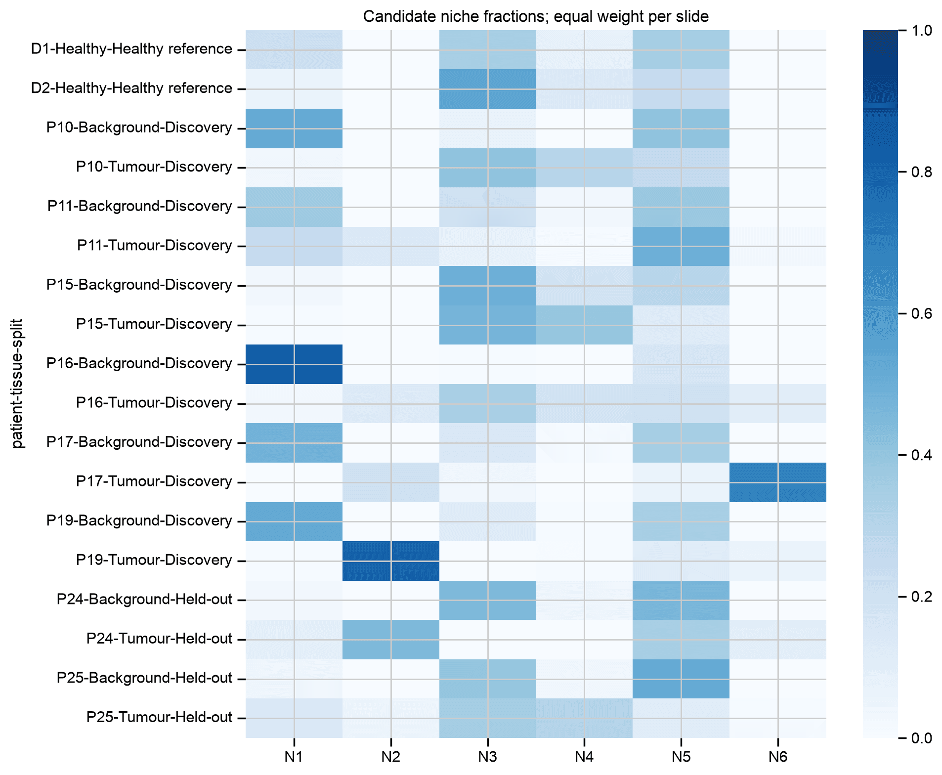
9a. Test tumour association in each held-out patient
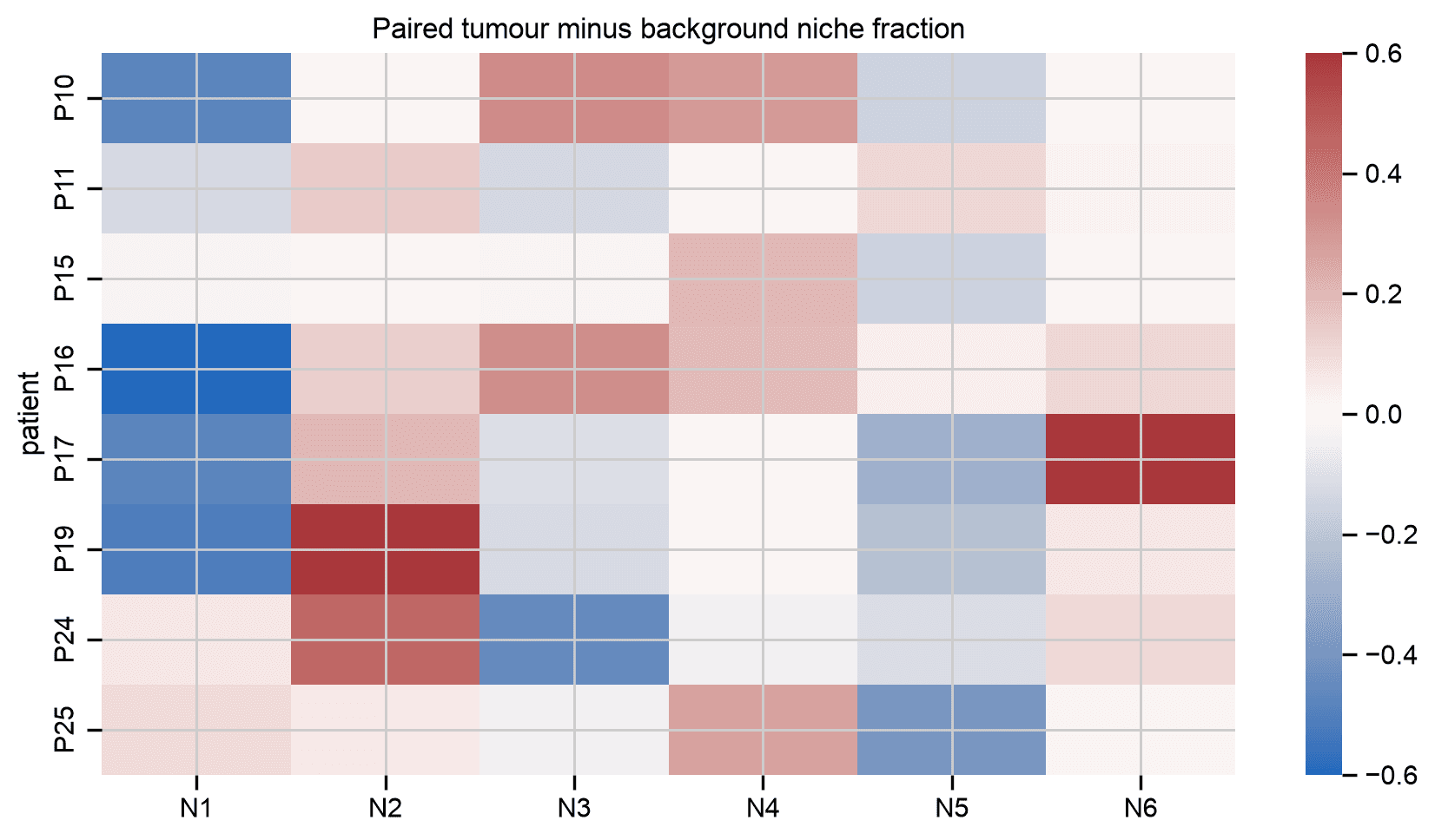
- Compute tumour-minus-background niche fractions within each patient.
- Pick candidate niches on discovery patients only: mean enrichment above 5 percentage points, and positive in at least four of six patients.
- A candidate passes in a held-out patient when it is tumour-enriched, has at least 50 spots across two slides, a marker-profile correlation of at least 0.5 with discovery, and state coverage of at least 0.8.
- These are fixed demo cutoffs, not significance tests.
tumour_fraction = patient_fractions.xs('Tumour', level='tissue').droplevel('split')
background_fraction = patient_fractions.xs('Background', level='tissue').droplevel('split')
paired_enrichment = tumour_fraction - background_fraction
candidate_niches = paired_enrichment.columns[
    (paired_enrichment.loc[DEVELOPMENT].mean() > 0.05)
    & (paired_enrichment.loc[DEVELOPMENT].gt(0).sum() >= 4)].tolist()
print('Discovery-selected tumour-associated candidates:', candidate_niches or 'None meet the stated rule')
display(paired_enrichment.round(3))
fig, ax = plt.subplots(figsize=(9, 5))
sns.heatmap(paired_enrichment, cmap='vlag', center=0, vmin=-0.6, vmax=0.6, ax=ax)
ax.set_title('Paired tumour minus background niche fraction')
plt.tight_layout(); plt.savefig(OUTPUT / 'paired_niche_enrichment.png', dpi=150); plt.show()

# First average within slide, then within patient; compare held-out patients separately.
by_patient_profile = profile_frame.groupby(
    ['patient_id', 'sample_id', 'spatial_niche'], observed=True)[score_cols].mean()
by_patient_profile = by_patient_profile.groupby(['patient_id', 'spatial_niche'], observed=True).mean()
discovery_profile = by_patient_profile.loc[DEVELOPMENT].groupby('spatial_niche', observed=True).mean()
support = data.obs.groupby(['patient_id', 'spatial_niche'], observed=True).agg(
    n_spots=('sample_id', 'size'), n_slides=('sample_id', 'nunique'),
    state_coverage=('state_in_reference', 'mean'), niche_coverage=('niche_in_reference', 'mean'))
transfer_rows = []
for patient in HOLDOUT:
    for niche in data.obs['spatial_niche'].cat.categories:
        if (patient, niche) not in support.index:
            transfer_rows.append({'patient_id': patient, 'niche': niche, 'supported': False,
                                  'n_spots': 0, 'n_slides': 0, 'marker_correlation': np.nan})
            continue
        stats = support.loc[(patient, niche)]
        supported = stats['n_spots'] >= 50 and stats['n_slides'] >= 2
        reference = discovery_profile.loc[niche].to_numpy()
        query = by_patient_profile.loc[(patient, niche)].to_numpy()
        correlation = np.corrcoef(reference, query)[0, 1] if supported else np.nan
        transfer_rows.append({'patient_id': patient, 'niche': niche,
                              **stats.to_dict(), 'supported': supported,
                              'marker_correlation': correlation,
                              'tumour_minus_background': paired_enrichment.loc[patient, niche],
                              'discovery_candidate': niche in candidate_niches})
niche_transfer = pd.DataFrame(transfer_rows)
display(niche_transfer.round(3))
Discovery-selected tumour-associated candidates: ['N2', 'N6']
            N1     N2     N3     N4     N5     N6
patient
P10     -0.477  0.000  0.337  0.294 -0.154  0.000
P11     -0.127  0.142 -0.135 -0.016  0.111  0.025
P15     -0.026  0.000 -0.021  0.206 -0.159  0.000
P16     -0.802  0.132  0.328  0.190  0.041  0.110
P17     -0.478  0.203 -0.112 -0.016 -0.287  0.689
P19     -0.515  0.803 -0.122 -0.004 -0.225  0.062
P24      0.062  0.451 -0.453 -0.046 -0.116  0.102
P25      0.097  0.058 -0.042  0.270 -0.399  0.017
   patient_id niche  n_spots  n_slides  state_coverage  niche_coverage  \
0         P24    N1    869.0       4.0           0.719           0.969
1         P24    N2   3124.0       4.0           0.923           0.999
2         P24    N3   2547.0       4.0           0.982           1.000
3         P24    N4    251.0       2.0           0.988           1.000
4         P24    N5   5024.0       4.0           0.771           0.952
5         P24    N6    702.0       2.0           0.963           0.999
6         P25    N1    614.0       4.0           0.879           0.907
7         P25    N2    161.0       2.0           1.000           1.000
8         P25    N3   2623.0       4.0           0.992           1.000
9         P25    N4    998.0       4.0           0.999           1.000
10        P25    N5   2449.0       4.0           0.928           0.956
11        P25    N6     47.0       2.0           1.000           1.000

    supported  marker_correlation  tumour_minus_background  \
0        True               0.857                    0.062
1        True               0.521                    0.451
2        True               0.276                   -0.453
3        True               0.176                   -0.046
4        True               0.256                   -0.116
5        True               0.929                    0.102
6        True               0.872                    0.097
7        True               0.445                    0.058
8        True               0.934                   -0.042
9        True               0.298                    0.270
10       True               0.874                   -0.399
11      False                 NaN                    0.017

    discovery_candidate
0                 False
1                  True
2                 False
3                 False
4                 False
5                  True
6                 False
7                  True
8                 False
9                 False
10                False
11 True 10Check spatial organisation
- Use the spot states, not the niches. Niches are built from neighbours, so neighbouring spots agree by construction.
- For each slide, compare how often neighbouring spots share a state with 100 shuffles of the state labels within that slide.
- Summarise per patient, because neighbouring spots aren't independent.
def spatial_state_enrichment(obs, adjacency, states, n_permutations, random_state):
    '''Share of neighbouring spots with the same state, against shuffles within each slide.'''
    rng = np.random.default_rng(random_state)
    states = np.asarray(states)
    edges = sparse.triu(adjacency, k=1).tocoo()
    slides = obs['sample_id'].astype(str).to_numpy()
    patients = obs['patient_id'].astype(str).to_numpy()
    rows = []
    for slide in np.unique(slides):
        nodes = np.flatnonzero(slides == slide)
        keep = slides[edges.row] == slide
        i, j = edges.row[keep], edges.col[keep]
        if len(i) == 0:
            continue
        observed = float(np.mean(states[i] == states[j]))
        shuffled = states.copy()
        null = []
        for _ in range(n_permutations):
            shuffled[nodes] = rng.permutation(states[nodes])
            null.append(np.mean(shuffled[i] == shuffled[j]))
        rows.append({'sample_id': slide, 'patient_id': patients[nodes[0]], 'n_edges': len(i),
                     'observed_same_state': observed, 'null_mean': float(np.mean(null)),
                     'null_sd': float(np.std(null)), 'excess': observed - float(np.mean(null))})
    return pd.DataFrame(rows)


spatial_results = spatial_state_enrichment(
    data.obs, discovery['adjacency'], discovery['states'],
    n_permutations=100, random_state=SEED,
)
display(spatial_results)
spatial_patient = spatial_results.groupby('patient_id').agg(
    observed=('observed_same_state', 'mean'),
    expected=('null_mean', 'mean'), excess=('excess', 'mean'))
display(spatial_patient)
sample_id patient_id n_edges observed_same_state null_mean null_sd \
0 D1_1 D1 346 0.456647 0.201994 0.021363
1 D1_2 D1 434 0.453917 0.232143 0.020641
2 D2_1 D2 4703 0.438444 0.239377 0.005631
3 D2_2 D2 6787 0.402240 0.283134 0.005524
4 P10_B1 P10 5041 0.555247 0.252672 0.006012
5 P10_B2 P10 5288 0.537254 0.278196 0.006155
6 P10_T1 P10 6306 0.643356 0.281541 0.005143
7 P10_T2 P10 5644 0.662651 0.294697 0.005956
8 P10_T3 P10 7439 0.586369 0.285135 0.004725
9 P10_T4 P10 7059 0.469613 0.218760 0.005669
10 P11_B1 P11 8233 0.427912 0.196933 0.004011
11 P11_B2 P11 8034 0.448345 0.206342 0.004346
12 P11_T1 P11 3057 0.472359 0.213948 0.006502
13 P11_T2 P11 3271 0.448487 0.193543 0.006724
14 P11_T3 P11 4768 0.496225 0.249799 0.005711
15 P11_T4 P11 4962 0.447400 0.255079 0.005730
16 P15_B1 P15 7919 0.430736 0.245993 0.004986
17 P15_B2 P15 7735 0.459341 0.287529 0.005336
18 P15_T1 P15 7313 0.560509 0.377119 0.005383
19 P15_T2 P15 8955 0.524176 0.321168 0.004103
20 P16_B1 P16 8786 0.493057 0.292367 0.004473
21 P16_B2 P16 9509 0.620360 0.416258 0.004817
22 P16_T1 P16 6464 0.436108 0.179500 0.004944
23 P16_T2 P16 6244 0.429212 0.171015 0.004677
24 P17_B1 P17 4149 0.487105 0.262099 0.006311
25 P17_B2 P17 2701 0.483525 0.251311 0.008144
26 P17_T1 P17 7544 0.725080 0.493368 0.004035
27 P17_T2 P17 8302 0.697422 0.455901 0.004658
28 P19_B1 P19 6220 0.504823 0.255672 0.005040
29 P19_B2 P19 6043 0.481549 0.242850 0.005412
30 P19_T1 P19 7156 0.654556 0.461582 0.004331
31 P19_T2 P19 6537 0.700780 0.541724 0.004196
32 P24_B1 P24 7491 0.412495 0.272452 0.005273
33 P24_B2 P24 8778 0.356573 0.248470 0.004264
34 P24_T1 P24 9914 0.346278 0.227705 0.003753
35 P24_T2 P24 10019 0.357820 0.213823 0.003439
36 P25_B1 P25 5655 0.410080 0.254329 0.004817
37 P25_B2 P25 6245 0.397278 0.261177 0.004664
38 P25_T1 P25 3679 0.494428 0.183487 0.005953
39 P25_T2 P25 4126 0.509210 0.203095 0.005814
excess
0 0.254653
1 0.221774
2 0.199067
3 0.119106
4 0.302575
5 0.259058
6 0.361814
7 0.367954
8 0.301234
9 0.250853
10 0.230979
11 0.242003
12 0.258410
13 0.254943
14 0.246426
15 0.192322
16 0.184743
17 0.171811
18 0.183390
19 0.203008
20 0.200690
21 0.204101
22 0.256607
23 0.258197
24 0.225006
25 0.232214
26 0.231711
27 0.241521
28 0.249151
29 0.238699
30 0.192974
31 0.159056
32 0.140043
33 0.108103
34 0.118573
35 0.143997
36 0.155751
37 0.136101
38 0.310940
39 0.306115 observed expected excess patient_id D1 0.455282 0.217069 0.238214 D2 0.420342 0.261255 0.159086 P10 0.575748 0.268500 0.307248 P11 0.456788 0.219274 0.237514 P15 0.493690 0.307952 0.185738 P16 0.494684 0.264785 0.229899 P17 0.598283 0.365670 0.232613 P19 0.585427 0.375457 0.209970 P24 0.368292 0.240613 0.127679 P25 0.452749 0.225522 0.227227
11Predict tissue in held-out patients
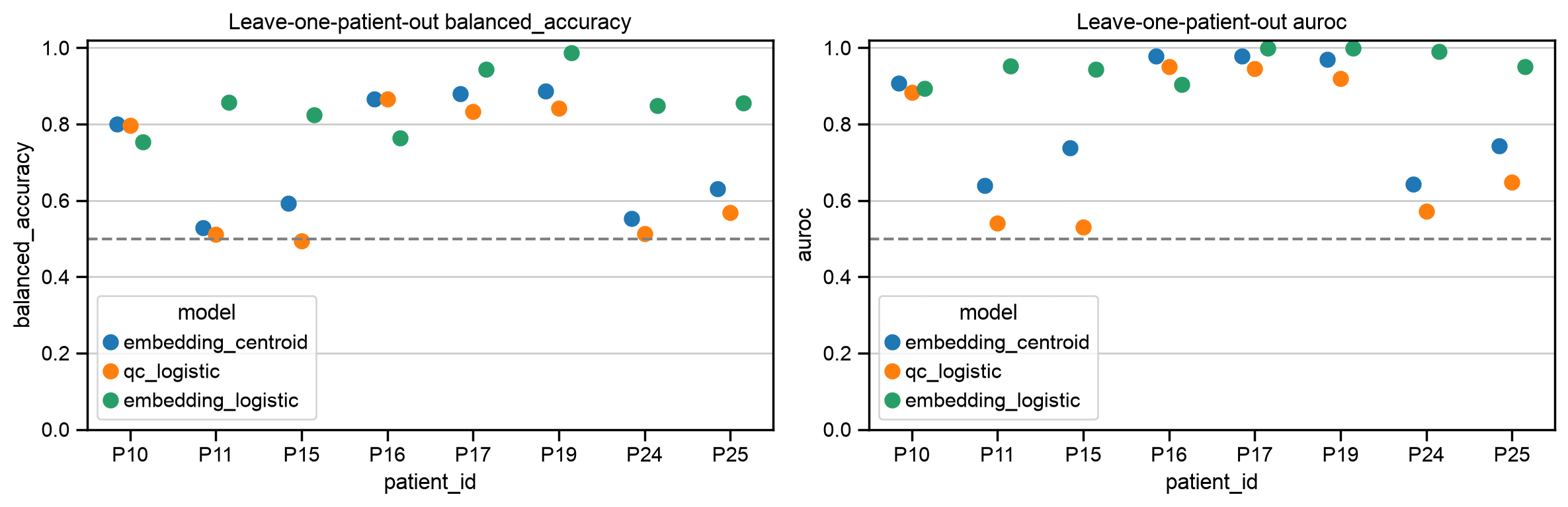
- Leave one patient out across the eight cancer patients. All slides from the held-out patient stay out of training.
- Fit a nearest-centroid readout and a logistic probe on the frozen Nicheformer embeddings. Compare both with a QC-only baseline: depth, detected genes and mitochondrial fraction.
- These steps use tissue labels, so they measure how much tissue signal the frozen embeddings carry. They aren't zero-shot predictions.
- A label-shuffle control swaps tumour and background within training patients. Chance is 0.5.
from sklearn.linear_model import LogisticRegression
from sklearn.metrics import balanced_accuracy_score, roc_auc_score
from sklearn.pipeline import make_pipeline
from sklearn.preprocessing import StandardScaler

QC_FEATURES = ['log1p_total_counts', 'n_genes_by_counts', 'pct_counts_mt']
TRAIN_PER_SLIDE = 500


def probe():
    return make_pipeline(StandardScaler(), LogisticRegression(max_iter=2000))


def centroid_scores(x_train, y_train, x_test):
    tumour, background = (normalize(x_train[y_train == k].mean(axis=0, keepdims=True)) for k in (1, 0))
    return (x_test @ (tumour - background).T).ravel()


def leave_one_patient_out(embedding, obs, n_permutations, random_state, include_logistic=True):
    '''Tumour versus background, holding out all slides of one cancer patient at a time.'''
    rng = np.random.default_rng(random_state)
    cancer = obs['tissue_group'].isin(['Tumour', 'Background']).to_numpy()
    x = normalize(embedding)
    qc = obs[QC_FEATURES].to_numpy(dtype=float)
    y = obs['tissue_group'].eq('Tumour').to_numpy().astype(int)
    patients = obs['patient_id'].astype(str).to_numpy()
    metrics, predictions, null = [], [], []
    for patient in sorted(np.unique(patients[cancer])):
        test = cancer & (patients == patient)
        train = balanced_sample(cancer & (patients != patient), obs, TRAIN_PER_SLIDE, rng)
        scores = {'embedding_centroid': centroid_scores(x[train], y[train], x[test]),
                  'qc_logistic': probe().fit(qc[train], y[train]).predict_proba(qc[test])[:, 1]}
        if include_logistic:
            scores['embedding_logistic'] = probe().fit(x[train], y[train]).predict_proba(x[test])[:, 1]
        for model, score in scores.items():
            threshold = 0 if model == 'embedding_centroid' else 0.5
            metrics.append({'patient_id': patient, 'model': model, 'n_spots': int(test.sum()),
                            'balanced_accuracy': balanced_accuracy_score(y[test], score > threshold),
                            'auroc': roc_auc_score(y[test], score)})
            predictions.append(pd.DataFrame({'spot_id': obs.index[test], 'patient_id': patient, 'model': model,
                                             'tumour': y[test], 'score': score}))
        # Control: swap tumour and background for a random half of the training patients.
        null_model = 'embedding_logistic' if include_logistic else 'embedding_centroid'
        for permutation in range(n_permutations):
            flipped = rng.choice(np.unique(patients[train]), size=len(np.unique(patients[train])) // 2, replace=False)
            y_null = np.where(np.isin(patients[train], flipped), 1 - y[train], y[train])
            if include_logistic:
                score = probe().fit(x[train], y_null).predict_proba(x[test])[:, 1]
                prediction = score > 0.5
            else:
                score = centroid_scores(x[train], y_null, x[test])
                prediction = score > 0
            null.append({'patient_id': patient, 'model': null_model, 'permutation': permutation,
                         'balanced_accuracy': balanced_accuracy_score(y[test], prediction),
                         'auroc': roc_auc_score(y[test], score)})
    null = pd.DataFrame(null)
    null_summary = null.groupby('model').agg(
        permutations=('permutation', 'nunique'),
        balanced_accuracy_mean=('balanced_accuracy', 'mean'), balanced_accuracy_sd=('balanced_accuracy', 'std'),
        auroc_mean=('auroc', 'mean'), auroc_sd=('auroc', 'std')).reset_index()
    return {'metrics': pd.DataFrame(metrics), 'predictions': pd.concat(predictions, ignore_index=True),
            'null_summary': null_summary}


evaluation = leave_one_patient_out(
    data.obsm['X_nicheformer'], data.obs,
    n_permutations=20, random_state=SEED,
)
patient_metrics = evaluation['metrics']
display(patient_metrics.round(3))
display(patient_metrics.groupby('model')[['balanced_accuracy', 'auroc']].agg(['mean', 'std']))
display(evaluation['null_summary'].round(3))
fig, axes = plt.subplots(1, 2, figsize=(12, 4))
for ax, metric in zip(axes, ['balanced_accuracy', 'auroc']):
    sns.pointplot(data=patient_metrics, x='patient_id', y=metric, hue='model',
                  dodge=0.3, errorbar=None, linestyles='none', ax=ax)
    ax.axhline(0.5, color='grey', linestyle='--')
    ax.set_ylim(0, 1.02)
    ax.set_title(f'Leave-one-patient-out {metric}')
plt.tight_layout(); plt.savefig(OUTPUT / 'heldout_patient_metrics.png', dpi=150); plt.show()
patient_id model n_spots balanced_accuracy auroc 0 P10 embedding_centroid 12872 0.800 0.907 1 P10 qc_logistic 12872 0.796 0.882 2 P10 embedding_logistic 12872 0.754 0.893 3 P11 embedding_centroid 11551 0.528 0.638 4 P11 qc_logistic 11551 0.511 0.541 5 P11 embedding_logistic 11551 0.857 0.952 6 P15 embedding_centroid 11423 0.592 0.738 7 P15 qc_logistic 11423 0.494 0.531 8 P15 embedding_logistic 11423 0.824 0.944 9 P16 embedding_centroid 10946 0.866 0.978 10 P16 qc_logistic 10946 0.866 0.951 11 P16 embedding_logistic 10946 0.764 0.903 12 P17 embedding_centroid 8226 0.880 0.978 13 P17 qc_logistic 8226 0.834 0.946 14 P17 embedding_logistic 8226 0.944 0.999 15 P19 embedding_centroid 9198 0.886 0.969 16 P19 qc_logistic 9198 0.841 0.920 17 P19 embedding_logistic 9198 0.986 1.000 18 P24 embedding_centroid 12517 0.554 0.643 19 P24 qc_logistic 12517 0.513 0.571 20 P24 embedding_logistic 12517 0.848 0.990 21 P25 embedding_centroid 6892 0.631 0.744 22 P25 qc_logistic 6892 0.569 0.649 23 P25 embedding_logistic 6892 0.856 0.950
                   balanced_accuracy               auroc
                                mean       std      mean       std
model
embedding_centroid          0.717019  0.155620  0.824412  0.149369
embedding_logistic          0.854106  0.080053  0.953955  0.041009
qc_logistic                 0.677934  0.169392  0.748915  0.192471
model permutations balanced_accuracy_mean \ 0 embedding_logistic 20 0.556 balanced_accuracy_sd auroc_mean auroc_sd 0 0.188 0.581 0.27
11a. Check sensitivity to low-count spots
- Repeat the comparison on spots that pass the QC flag (at least 500 UMIs and 200 detected genes).
- The embeddings are subset after alignment; Nicheformer isn't rerun.
qc_mask = data.obs['qc_pass'].to_numpy()
qc_evaluation = leave_one_patient_out(
    data.obsm['X_nicheformer'][qc_mask], data.obs.loc[qc_mask],
    n_permutations=20, random_state=SEED, include_logistic=True,
)
qc_metrics = qc_evaluation['metrics']
display(qc_metrics.round(3))
display(qc_metrics.groupby('model')[['balanced_accuracy', 'auroc']].mean().round(3))
patient_id model n_spots balanced_accuracy auroc 0 P10 embedding_centroid 11536 0.785 0.884 1 P10 qc_logistic 11536 0.775 0.847 2 P10 embedding_logistic 11536 0.773 0.943 3 P11 embedding_centroid 9361 0.506 0.618 4 P11 qc_logistic 9361 0.500 0.476 5 P11 embedding_logistic 9361 0.852 0.954 6 P15 embedding_centroid 11295 0.598 0.759 7 P15 qc_logistic 11295 0.487 0.511 8 P15 embedding_logistic 11295 0.716 0.916 9 P16 embedding_centroid 6809 0.850 0.967 10 P16 qc_logistic 6809 0.833 0.909 11 P16 embedding_logistic 6809 0.758 0.898 12 P17 embedding_centroid 7667 0.861 0.977 13 P17 qc_logistic 7667 0.816 0.932 14 P17 embedding_logistic 7667 0.954 0.998 15 P19 embedding_centroid 7818 0.856 0.964 16 P19 qc_logistic 7818 0.810 0.892 17 P19 embedding_logistic 7818 0.980 1.000 18 P24 embedding_centroid 11711 0.573 0.695 19 P24 qc_logistic 11711 0.534 0.598 20 P24 embedding_logistic 11711 0.835 0.993 21 P25 embedding_centroid 6486 0.686 0.825 22 P25 qc_logistic 6486 0.635 0.716 23 P25 embedding_logistic 6486 0.860 0.958
                    balanced_accuracy  auroc
model
embedding_centroid              0.714  0.836
embedding_logistic              0.841  0.958
qc_logistic                     0.674  0.735
12Summarise the results
- Read three views together: tissue signal in held-out patients, spatial organisation, and niches that recur with similar markers.
- Compare each one with the QC-only baseline and the label-shuffle control.
# This compact report is populated only from computed outputs.
means = patient_metrics.groupby('model')[['balanced_accuracy', 'auroc']].mean()
display(Markdown('**Measured evidence:**'))
display(means.round(3))
heldout_coverage = discovery['coverage'].loc[discovery['coverage']['patient_id'].isin(HOLDOUT)]
display(heldout_coverage)
transfer_check = niche_transfer.assign(passes=lambda f:
    f['supported'] & f['tumour_minus_background'].gt(0)
    & f['marker_correlation'].ge(0.5) & f['state_coverage'].ge(0.8))
recurrent_niches = [niche for niche in candidate_niches
                   if transfer_check.loc[transfer_check['niche'].eq(niche), 'passes'].sum() == len(HOLDOUT)]
centroid_ba = means.loc['embedding_centroid', 'balanced_accuracy']
probe_ba = means.loc['embedding_logistic', 'balanced_accuracy']
qc_ba = means.loc['qc_logistic', 'balanced_accuracy']
patient_range = patient_metrics.query("model == 'embedding_logistic'")['balanced_accuracy']
spatial_excess = float(spatial_patient['excess'].mean())
summary = (
    f'**Answer in this cohort.** Across eight patient-held-out folds, mean balanced accuracy '
    f'was **{centroid_ba:.3f}** for the Nicheformer centroid readout and **{probe_ba:.3f}** '
    f'for the supervised linear probe, versus **{qc_ba:.3f}** for QC alone. '
    f'Probe accuracy ranged from {patient_range.min():.3f} to {patient_range.max():.3f} across patients. '
    f'Across all ten subjects (including the two healthy donors), the mean excess of same-state physical neighbours over shuffled labels was '
    f'**{spatial_excess:.3f}**. Of {len(candidate_niches)} discovery-selected tumour-enriched '
    f'candidate niches, **{len(recurrent_niches)}** passed the stated exploratory transfer checks '
    f'in both held-out patients ({", ".join(recurrent_niches) or "none"}).'
)
interpretation = (
    'The combined results provide exploratory support for recurring tumour-associated spatial niches '
    'in frozen Nicheformer representations, with the patient-specific limitations shown above.'
    if recurrent_niches and probe_ba > qc_ba and spatial_excess > 0 else
    'The combined results do not establish reliable recovery of tumour-associated niches across '
    'both held-out patients under the stated checks; examine which component failed in the tables above.'
)
display(Markdown(summary + '\n\n' + interpretation +
    ' These spot mixtures are not validated malignant or immune-cell identities. A counts-derived '
    'baseline and independent spatial annotations are still needed to establish model-specific added value.'))
(OUTPUT / 'findings.md').write_text(summary + '\n\n' + interpretation + '\n')
<IPython.core.display.Markdown object>
                    balanced_accuracy  auroc
model
embedding_centroid              0.717  0.824
embedding_logistic              0.854  0.954
qc_logistic                     0.678  0.749
  patient_id     split  spots  state_coverage  niche_coverage
8        P24  Held-out  12517        0.863466        0.978429
9        P25  Held-out   6892        0.960389        0.976204
<IPython.core.display.Markdown object>
757
What the recorded run shows
- Tissue signal transfers across patients. The logistic probe on Nicheformer embeddings reaches a mean balanced accuracy of 0.854 across the eight held-out folds, against 0.678 for the QC-only baseline and 0.717 for the nearest-centroid readout. The label-shuffle control stays near chance (0.556).
- N2 is the strongest candidate niche. It is tumour-enriched in both held-out patients (+45.1 and +5.8 percentage points) and is built mostly from the myeloid- and hypoxia-high state S1. Its marker correlation is 0.521 in P24 but 0.445 in P25, just under the 0.5 cutoff.
- N6 can't be tested in P25. It passes every check in P24 (+10.2 points, marker correlation 0.929), but P25 has only 47 N6 spots, below the 50-spot cutoff. The same niche label doesn't guarantee the same support in every patient.
- Some structure is technical. State S2 has a median of 181 UMIs and almost none of its spots pass the QC flag, and niche N1 is dominated by S2 and the low-count state S8.
- Confirming specific microenvironments needs pathology or cell-composition labels, and a counts-derived baseline to isolate what Nicheformer adds.
13Save the results
- Save a compact AnnData with annotations, embeddings, UMAP, states, niches and physical neighbours. Counts and images stay in the source files.
- Save the result tables as CSV and the fitted state and niche models.
- Keep the downloaded embeddings: repeating the analysis needs no new run.
import joblib

result = ad.AnnData(X=sparse.csr_matrix((data.n_obs, 0)), obs=data.obs.copy())
for key in ['X_nicheformer', 'X_umap', 'spatial', 'state_neighborhood_proportions']:
    result.obsm[key] = data.obsm[key]
result.obsp['physical_neighbors'] = data.obsp['physical_neighbors']
result.uns['source_h5ad'] = str(INPUT)
result.uns['development_patients'] = DEVELOPMENT
result.uns['heldout_patients'] = HOLDOUT
result.write_h5ad(OUTPUT / 'spatial_nicheformer_analysis.h5ad', compression='gzip')
patient_metrics.to_csv(OUTPUT / 'patient_metrics.csv', index=False)
evaluation['null_summary'].to_csv(OUTPUT / 'patient_label_shuffle_control.csv', index=False)
spatial_results.to_csv(OUTPUT / 'spatial_state_enrichment.csv', index=False)
patient_fractions.to_csv(OUTPUT / 'niche_patient_fractions.csv')
state_profiles.to_csv(OUTPUT / 'state_marker_profiles.csv')
niche_profiles.to_csv(OUTPUT / 'niche_marker_profiles.csv')
paired_enrichment.to_csv(OUTPUT / 'paired_niche_enrichment.csv')
niche_transfer.to_csv(OUTPUT / 'heldout_niche_transfer.csv', index=False)
qc_metrics.to_csv(OUTPUT / 'qc_sensitivity_patient_metrics.csv', index=False)
evaluation['predictions'].to_csv(OUTPUT / 'out_of_fold_predictions.csv', index=False)
discovery['coverage'].to_csv(OUTPUT / 'reference_coverage.csv', index=False)
joblib.dump(discovery['models'], OUTPUT / 'frozen_state_niche_models.joblib')
(OUTPUT / 'analysis_settings.json').write_text(json.dumps({
    'seed': SEED, 'development': DEVELOPMENT, 'holdout': HOLDOUT,
    'state_count': 8, 'niche_count': 6, 'programs': programs,
    'source': str(INPUT),
    'versions': {p: importlib.metadata.version(p) for p in
                 ['anndata', 'scanpy', 'numpy', 'pandas', 'scikit-learn']},
}, indent=2))
print(f'Results and figures saved to {OUTPUT}')
Results and figures saved to results
Takeaways
- The Helical MCP handles registration, the Nicheformer run and the download. You choose the patient split, the analysis and the controls.
- The same workflow works for other models on the platform: change the model name in the prompt for step 3b.
- Score a simple baseline next to the model (here, QC covariates), so each number has a reference point.
- Split by patient, not by spot, when you test whether results transfer to new patients.
- This analysis is one of many computational experiments you can run in Helical, the virtual AI lab for biology.
References
- De Zuani M, et al. Single-cell and spatial transcriptomics analysis of non-small cell lung cancer. Nature Communications 2024;15:4388. 10.1038/s41467-024-48700-8
- Spatial data: E-MTAB-13530
- Tejada-Lapuerta A, Schaar AC, et al. Nicheformer: a foundation model for single-cell and spatial omics. Nature Methods 2025;22:2525–2538. 10.1038/s41592-025-02814-z
- Nicheformer code: official implementation and Helical implementation